Fast Fourier transform (FFT)

Next: Misc. commands Up: DSP functions Previous: Frequency response

Fast Fourier transform (FFT)

Best way to explain that is using an example. Assume that we have a sinusoidal signal that we want to determine its Fourier transform.

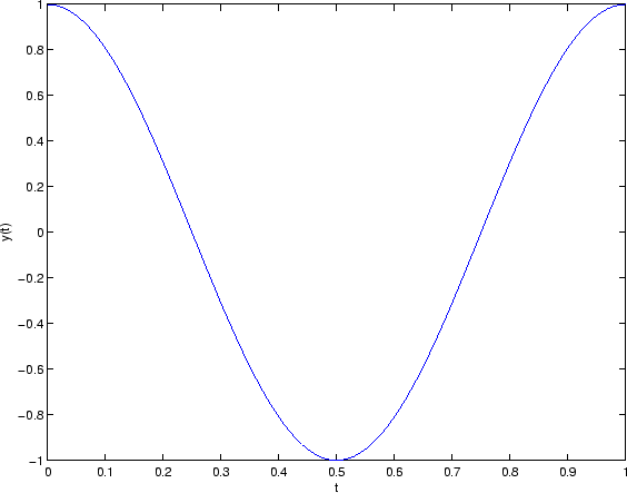
>> fs=100;
>> t=0:1/fs:1;
>> y=cos(2*pi*t);
>> plot(t,y)
>> xlabel('t')
>> ylabel('y(t)')

**Figure 9:** 1sec sinwave of 1Hz
$\begin{figure} \center \epsfig{width=5in,file=fft_cos_1sec.eps} \end{figure}$

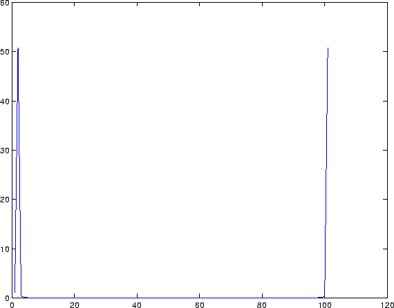
Use the following commands to compute the FFT, find its length and plot the magnitude of .

>> Y=fft(y);
>> length(Y)

ans =

   101

>> plot(abs(Y))

**Figure 10:** 101-point FFT
$\begin{figure} \center \epsfig{width=5in,file=fft_absY_1sec_101.eps} \end{figure}$

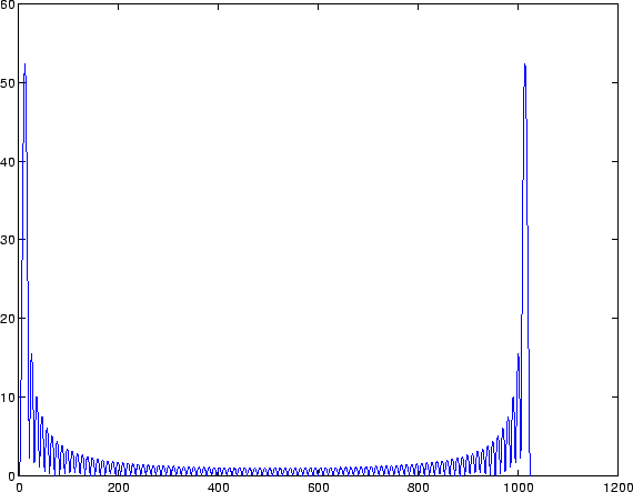
The above plot doesn't show many details since it is only using 101 points. We can specify the length of the FFT to be longer by

>> N=1024;
>> Y=fft(y,N);
>> plot(abs(Y))

**Figure 11:** 1024-point FFT
$\begin{figure} \center \epsfig{width=5in,file=fft_absY_1sec_1024.eps} \end{figure}$

Now we can see more details, but still we can't extract a lot of information from the plot. If we compute the Fourier transform of a sine or a cosine function we expect to see two impulses at the frequency of the sine or the cosine. But, that's not what we are seeing. Here is how we can modify the plot to see something more familiar.

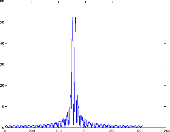
>> plot(fftshift(abs(Y)))

**Figure 12:** `fftshift`
$\begin{figure} \center \epsfig{width=5in,file=fft_absY_1sec_1024_fftshift.eps} \end{figure}$

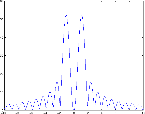
If we zoom around the center we get something familiar.

**Figure 13:** `fftshift` zoomed
$\begin{figure} \center \epsfig{width=5in,file=fft_absY_1sec_1024_fftshift_zoom.eps} \end{figure}$

But, it is not really the impulses that we expected. We have all those ripples and also the x-axis does not match the frequency of the $\cos$ . Let's deal with the second problem first.

We need to map the x-axis value to reflect frequency in Hz. To do that all you need to remember that the length of the FFT corresponds to the sampling rate for continuous frequencies and corresponds to $2\pi$ for discrete frequency. Therefore to get the positive and negative frequencies you need to get the following.

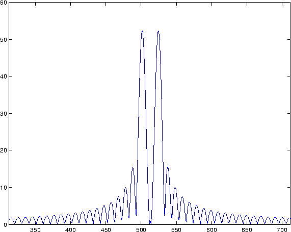
>> k=-N/2:N/2-1;
>> plot(k,fftshift(abs(Y)))

**Figure 14:** `fftshift` with
$\begin{figure} \center \epsfig{width=5in,file=fft_absY_1sec_1024_fftshift_k.eps} \end{figure}$

Now we get the axis containing positive and negative values. All we have left to do is to map it to actual frequencies.

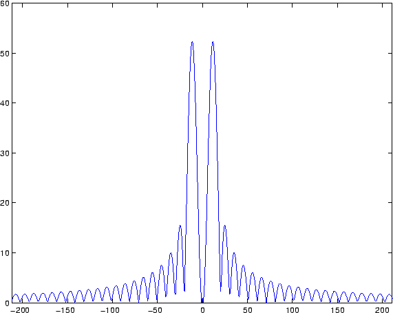
>> plot(k*fs/N,fftshift(abs(Y)))

**Figure 15:** Frequency mapping
$\begin{figure} \center \epsfig{width=5in,file=fft_absY_1sec_1024_fftshift_f.eps} \end{figure}$

Now are getting something meaningful. We have the two peaks at $\pm 1$ Hz. But, they are not really impulses like we wanted. The reason is we really wanted an infinitly long sinusoide to get the impulses, due to the fact that we can't have an infinitly long sinusoide to process, we have effectively multiplied the sinusoid by a rectangular window of length 1sec. If we multiply in the time domain by a rectangular window, we convolve in the frequency domain with a sinc function. That is what we are getting, two sinc functions centered around $\pm 1$ Hz.

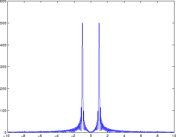
If we increase the length of the window, we expect the sinc function to look more and more like an impulse. To do that lets generate a sinusoidal signal that last for 10sec instead.

>> fs=100;
>> t=0:1/fs:10;
>> y=cos(2*pi*t);
>> N=4096;
>> Y=fft(y,N);
>> k=-N/2:N/2-1;
>> plot(k*fs/N,fftshift(abs(Y)))

**Figure 16:** FFT of a 10sec 1Hz sinwave
$\begin{figure} \center \epsfig{width=5in,file=fft_absY_1sec_1024_fftshift_f_long.eps} \end{figure}$

Next: Misc. commands Up: DSP functions Previous: Frequency response