EE 101 - Lab 4:  PSPICE Evaluation of an RC Network

Prelab Exercises

ALL GRAPHS MUST BE FULLY LABELED AND DRAWN NEATLY!

 NO ANSWERS ARE COMPLETE WITHOUT THE UNITS! AS ALWAYS, SHOW YOUR WORK!


Circuit for prelab exercises

For parts 1, 2, and 3, assume the switch has been in position 1 for a long time. At t = 0s, the switch moves to position 2 and the capacitor begins to charge.

For part 3, assume the switch has been closed for a long time. At t = 0s, the switch is opened and the capacitor begins to discharge.

  1. Draw the charge curve for the capacitor using the 2/3 estimation method given in class.

  2.  
  3. Answer the following:

  4.  
    1. What is the time constant for the circuit?

    2.  
    3. What will the capacitor voltage be at t = 150 ns?

    4.  
    5. What will the resistor voltage be at t = 150 ns?

    6.  
    7. What will the resistor current be at t = 150 ns?

    8.  
    9. How much time must pass for the capacitor voltage to reach 1 volt?

    10.  
  5. Draw the charge curve using the capacitor charge formula given in class.

  6.  
  7. Assume the capacitor is fully charged, and the switch moves to position 1 at t = 0s. Draw the discharge curve using the capacitor discharge formula given in class.

  8. (end of pre-lab)


Lab Exercise 4: PSPICE  Evaluation of an RC Network

The purpose of this lab is to analyze an RC network using PSPICE.
  1. Enter the following circuit (Figure 1) into the PSPICE schematic editor.

  2.  


     Figure 1

    Unlike in  last week's simulation, the voltage source you will use today will be a 0 to 5v pulse signal (Vpulse). The purpose of the pulse is to model a switch opening and closing. When the pulse is low (0 volts), the switch is modeled as open and when the pulse is high (5 volts), the switch is modeled as closed. You will need to define the parameters of the pulse. For the purpose of this exercise, you will inject a waveform that is 5 volts for the first 500 ns and 0 volts for the next 500 ns. To accomplish this, double click on the Vpulse symbol and enter the following attributes: V1 = 0V, V2 = 5V, TD = 0, TR = 0, TF = 0, PW = 0.5us, and PER = 1us. (TR = risetime, TF = falltime, TD = delay time, PW = pulse width, and PER = period of waveform)

    Notice there are two voltage level markers on the schematic. These are used in the probe feature of PSPICE. Probe allows the user to observe how a circuit affects a signal. Specifically, you will observe how a 5 volt source charges the capacitor in an RC network (and how the capacitor discharges in the same network). Place the voltage markers on your schematic--one to measure the source voltage and one to measure the capacitor voltage (under the Markers menu, choose Mark Voltage/Level).

    Before you simulate this circuit, make sure your analysis setup is correct. Under the Analysis menu, go to Setup and check to see that the Bias Point Detail and Transient options are enabled.

    Perform an Electrical Rule Check and simulate your circuit. After a bit, the MicroSim Probe window will appear. It should look like this (Figure 2).
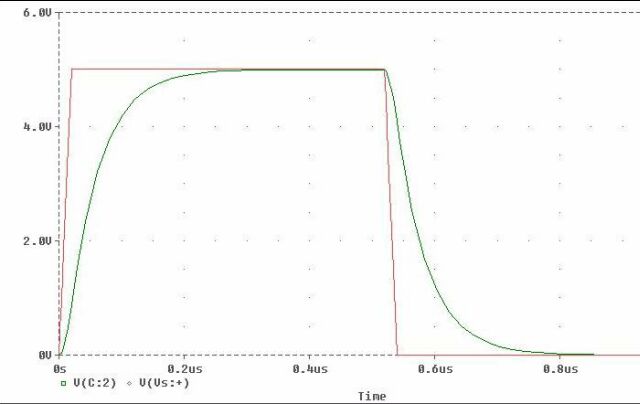
     Figure 2

    Notice that while the pulse reads 5 volts from 0 s to 500 ns, the capacitor is shown to be charging, while during the low portion of the pulse wave (500 ns to 1 us) the capacitor is discharging.

    Add a set of cursors to the probe output (Tools - Cursor - Display). Click the right mouse button to display one set of vertical crosshairs. To make these crosshairs stick to the capacitor voltage curve, go down to the curve label (V(C:2)) and use the same mouse button to click on the small diamond to the left of the label. In the same way, but using the left mouse button, add the second cursor. This time, click on the diamond with the left mouse button to make the cursor stick to the charging curve.
     

    1. A rule of thumb states that the time it takes for a capacitor to charge from 10% to 90% of its maximum value is approximately equal to 2.2 times the time constant for that curve. Using the left mouse button to control one, and the right button to control the other, move one set of cursors to 0.5 volts (10% of 5 volts) and the other to 4.5 volts (90% of 5 volts). Keep track of the voltage value the cursor is at by watching the Probe Cursor box at the bottom of the probe window. When you are close to 0.5 and 4.5 volts, take note of the elapsed time difference between them. Divide this time value by 2.2. Does this number basically agree with the RC time constant value you calculated in the pre-lab?

    2.  
    3. Leaving one cursor at the origin, position the second cursor at the 150 ns mark. Read the capacitor voltage at this point. Does this value agree with what you calculated in part 2b of the pre-lab?

    4.  
    5. Leaving the cursors as they are (in 1b), label your plot (Tools - Label - Text) first with "RC = 50 ns" and then with your name. Neatly place this information under the charging curve. Next, you will print out the plot. To keep from using an entire piece of paper for the print job, go to File-Print and then click on the Page Setup button. Locate Plots Per Page and choose 4. Then print out the plot and tape it into your lab book.

    6.  
  3. Using what you know about the series and parallel relationships of resistors and capacitors, reduce the schematic in Figure 3 to a circuit with a single equivalent resistor and capacitor. Fully label your schematic.

  4.  
    1. What is the RC time constant for the circuit?

    2.  
    3. Sketch the capacitor charging and discharging curves using the 2/3 approximation method. Fully label your plots.

    4.  


      Figure 3

  5. Enter the circuit in Figure 3 into the schematic editor in PSPICE.

  6.  
    1. For Vs, configure a pulse signal with a 40 volt peak amplitude that is 150 ns in length. Use a period of 300 ns, along with rise, fall, and delay times of 0 s. Place voltage level markers at the appropriate nodes to measure the input pulse and the voltage across the equivalent capacitance. Under the Draw menu, use Text to place your name in your circuit. Save your drawing, print out a copy (make it small enough to fit nicely in your lab book!), and tape it into your lab book.

    2.  
    3. Perform an electrical rules check on your circuit, set up probe to run a transient analysis, and simulate your circuit as before.

    4. When your probe results are displayed, notice that the input pulse is repeated until it gets to the 1.0 us mark. Your first simulation you ran today used up the same amount of time, as well. However, that pulse was of a lower frequency and thus took up the entire span. Over three of the present pulses can fit in the 1.0 us time span because it is of shorter duration.

      Like before, determine the time constant for this circuit by using the 10% to 90% risetime method. Print out a copy of your plot that shows the cursors in the 10% and 90% of total voltage amplitude positions. On this plot, add a label with the time constant information and your name. Tape the printout into your lab book.


    January 2001

    Copyright 2001, New Mexico Tech