EE212 Matlab Example: System Frequency Response
Matlab m-file:
% File Name: example2.m
%
% Description: Matlab m-file for plotting a frequency response of class example III.B.14. using
% a) standard plotting and complex number capabilities,
% b) standard plotting and complex number capabilities for generating Bode plots, and
% c) built in Bode plot function.
% Transfer function:
2500(10 + jw)
%
H(jw) = ----------------------------------
%
jw(2 + jw)(2500 + jw30 + (jw)^2)
% clear matlab memory and close all open figures
clear all; close all;
%=======================================================================================
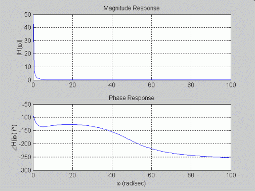
% a) plotting of frequency response using standard complex number and plotting functions
%=======================================================================================
% open figure 1 for first frequency response plots
figure(1);
% create vector of 200 equally spaced frequencies from 0.1rad/sec to 100rad/sec
% note 0rad/sec is not used because it causes a divide by zero (jw=0 is a pole)
w = linspace(0.1,100,200);
% define transfer function
H = 2500*(10+j*w)./(j*w.*(2+j*w).*(2500+j*w*30+(j*w).^2));
% divide figure window into two rows, one column, and plot magnitude response in top graph,
% phase response in bottom graph
subplot(2,1,1);
plot(w,abs(H));
grid; ylabel('|H(j\omega)|'); title('Magnitude Response');
subplot(2,1,2);
plot(w,unwrap(angle(H))*180/pi);
grid; xlabel('\omega (rad/sec)'); ylabel('\angleH(j\omega) (\circ)'); title('Phase Response');
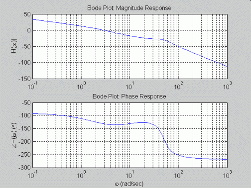
%=======================================================================================
% b) plotting of frequency response as a Bode plot using standard complex number
% and plotting functions
%=======================================================================================
% open figure 2 for second frequency response plots
figure(2);
% create vector of 200 logarithmically spaced (i.e., same number of points per decade)
% frequencies from 10^-1 = 0.1rad/sec to 10^3 = 1000rad/sec
w = logspace(-1,3,200);
% define transfer function
H = 2500*(10+j*w)./(j*w.*(2+j*w).*(2500+j*w*30+(j*w).^2));
% divide figure window into two rows, one column, and plot magnitude response in top graph,
% phase response in bottom graph
subplot(2,1,1);
semilogx(w,20*log10(abs(H)));
grid; ylabel('|H(j\omega)|'); title('Bode Plot: Magnitude Response');
subplot(2,1,2);
semilogx(w,unwrap(angle(H))*180/pi);
grid; xlabel('\omega (rad/sec)'); ylabel('\angleH(j\omega) (\circ)'); title('Bode Plot: Phase Response');
%=======================================================================================
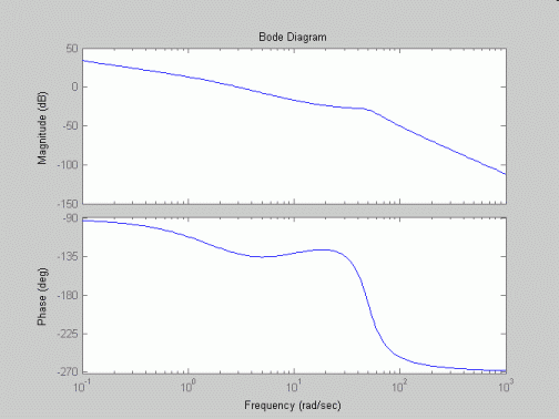
% c) plotting of frequency response using Bode function
%=======================================================================================
% open figure 3 for third frequency response plots
figure(3);
% create vector of 200 logarithmically spaced (i.e., same number of points per decade)
% frequencies from 10^-1 = 0.1rad/sec to 10^3 = 1000rad/sec
w = logspace(-1,3,200);
% define transfer function using coefficients of jw in numerator and denominator
% starting with highest power of jw and working down - note conv() is used to
% multiply terms in denominator
numH = 2500*[1 10];
denH = conv([1 0], conv([1 2], [1 30 2500]));
% call bode() to plot frequency response as bode diagrams, then add grids
bode(numH,denH,w);
Procedure for running m-file: change working directory to where m-file is stored and then enter m-file name at command prompt.
>> pwd
ans =
C:\matlabR12\work
>> cd ../../temp/ee212/
>> dir
.                 example1.html     example1fig1.gif  example1fig3.gif  example2.m
..                example1.m        example1fig2.gif  example2.html
>> example2
>>
Plots generated: