% EE 212 Example 4
% Description:  M-file showing several methods of plotting
% the frequency response of a simple RC circuit with
% transfer function H(s) = (1/RC)/(s + 1/RC).
%
% Here R = 10kOhm, C = 1uF => 1/RC = 100.

% Clear Matlab memory, clear command window, close all existing figures
clear; clc; close all;

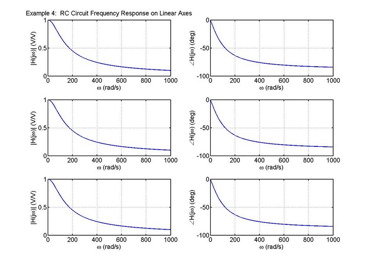
%===== Frequency response on linear axes =====
figure(1); % open first figure
% 1001 linearly spaced frequencies from 0 to 1000rad/sec
wlin = linspace(0,1000,1001);

% Compute and plot magnitude and phase of TF
Hmag1 = 100./sqrt(100^2+wlin.^2);
Hpha1 = -atan2(wlin,100)*180/pi;
subplot(3,2,1);
plot(wlin,Hmag1); xlabel('\omega (rad/s)'); ylabel('|H(j\omega)| (V/V)');
title('Example 4:  RC Circuit Frequency Response on Linear Axes'); grid;
subplot(3,2,2);
plot(wlin,Hpha1); xlabel('\omega (rad/s)'); ylabel('\angleH(j\omega) (deg)'); grid;

% Compute TF and plot its magnitude (via abs()) and phase (via angle())
H2     = 100./(j*wlin + 100);
Hmag2  = abs(H2);
Hpha2  = angle(H2)*180/pi;
subplot(3,2,3);
plot(wlin,Hmag2); xlabel('\omega (rad/s)'); ylabel('|H(j\omega)| (V/V)'); grid;
subplot(3,2,4);
plot(wlin,Hpha2); xlabel('\omega (rad/s)'); ylabel('\angleH(j\omega) (deg)'); grid;

% Compute TF via bode() and plot its magnitude and phase
% Define coefficients of powers of s in numerator and denominator
numH = [100]; denH = [1, 100];
% Call bode()
[Hmag3,Hpha3] = bode(numH,denH,wlin);
subplot(3,2,5);
plot(wlin,Hmag3); xlabel('\omega (rad/s)'); ylabel('|H(j\omega)| (V/V)'); grid;
subplot(3,2,6);
plot(wlin,Hpha3); xlabel('\omega (rad/s)'); ylabel('\angleH(j\omega) (deg)'); grid;

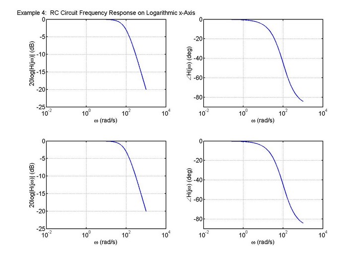
%===== Frequency response on logarithmic axes with magnitude in dB =====
figure(2); % open second figure

% 1000 logrithmically spaced frequencies from 10^(-1) to 10^3 rad/sec
wlog    = logspace(-1,3,1000);

H4      = 100./(j*wlog + 100);
Hmag4dB = 20*log10(abs(H4));
Hpha4   = angle(H4)*180/pi;
subplot(2,2,1);
semilogx(wlog,Hmag4dB); xlabel('\omega (rad/s)'); ylabel('20log|H(j\omega)| (dB)'); grid;
title('Example 4:  RC Circuit Frequency Response on Logarithmic x-Axis'); 
subplot(2,2,2);
semilogx(wlog,Hpha4); xlabel('\omega (rad/s)'); ylabel('\angleH(j\omega) (deg)'); grid;

% Define coefficients of powers of s in numerator and denominator
[Hmag5,Hpha5] = bode(numH,denH,wlog);
subplot(2,2,3);
semilogx(wlog,20*log10(Hmag5)); xlabel('\omega (rad/s)'); ylabel('20log|H(j\omega)| (dB)'); grid;
subplot(2,2,4);
semilogx(wlog,Hpha5); xlabel('\omega (rad/s)'); ylabel('\angleH(j\omega) (deg)'); grid;

>> example4

Figures/Plots Generated: