Plotting Trigonometric Fourier Series using Matlab

M-file:

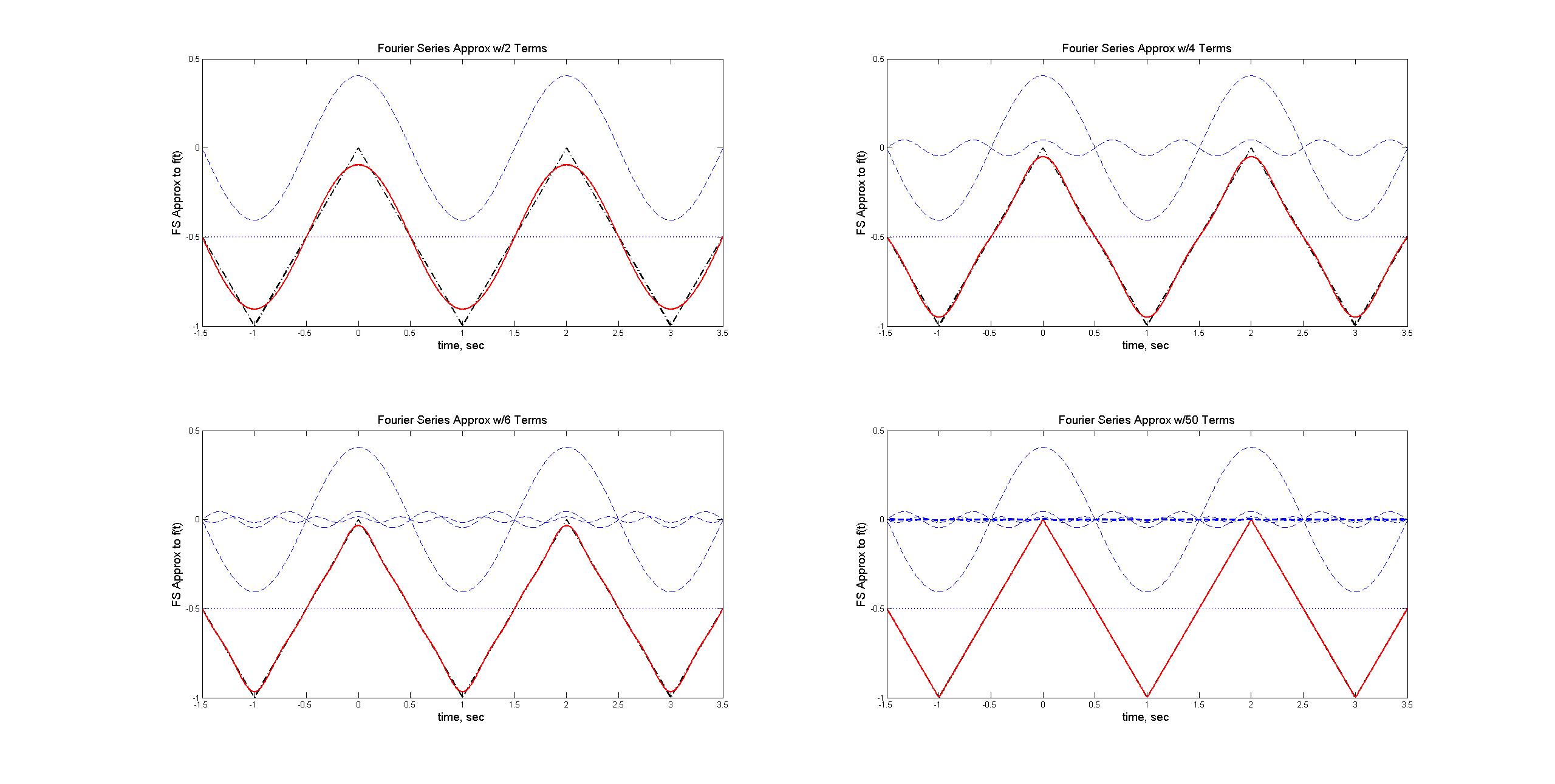
        %% Filename: FourierSeriesExample5.m
        % Description: m-file to plot trigonometric Fourier Series
        % representation of a triangle wave.
        
        clear; clc; close all; % clear memory and command window, close all figures
        
        t = -1.5:0.005:3.5; % times over which to plot FS
        
        Nval = [2, 4, 6, 50]; % upper limits for n in summation
        
        figure(1); % open figure in which to plot
        
        % Build triangle wave using increasing number of terms
        for in = 1:4, % loop over 4 different lengths (found in Nval) of Fourier Series
          f = -1/2*ones(1,length(t)); % a0 (DC offset) term
          subplot(2,2,in); % open one of four subplots
          % brute force original triangle wave
          plot([-1.5, -1, 0, 1, 2,  3, 3.5],...
          [-0.5, -1, 0,-1, 0, -1,-0.5],'k-.','LineWidth',2);
          hold on;
          plot(t,f,'b:','LineWidth',2); % plot a0 (DC offset)
          for n = 1:2:Nval(in), % loop over different lengths of FS
            harm = 4*cos(n*pi*t)/(n*n*pi*pi); % compute terms (harmonics)
            f    = f + harm; % add terms to series
            plot(t,harm,'b--','LineWidth',1); % plot terms (harmonics)
          end
          plot(t,f,'r-','LineWidth',2); % plot FS
          hold off;
          xlabel('time, sec','FontSize',14); ylabel('FS Approx to f(t)','FontSize',14);
          title(['Fourier Series Approx w/',num2str(Nval(in)),' Terms'],'FontSize',14);
        end
      

Figures/Plots Generated: