Plotting Complex (Exponential) Fourier Series using Matlab

M-file:

        %% Filename: FourierSeriesExample6.m
        % Description: m-file to plot complex (exponential) Fourier Series
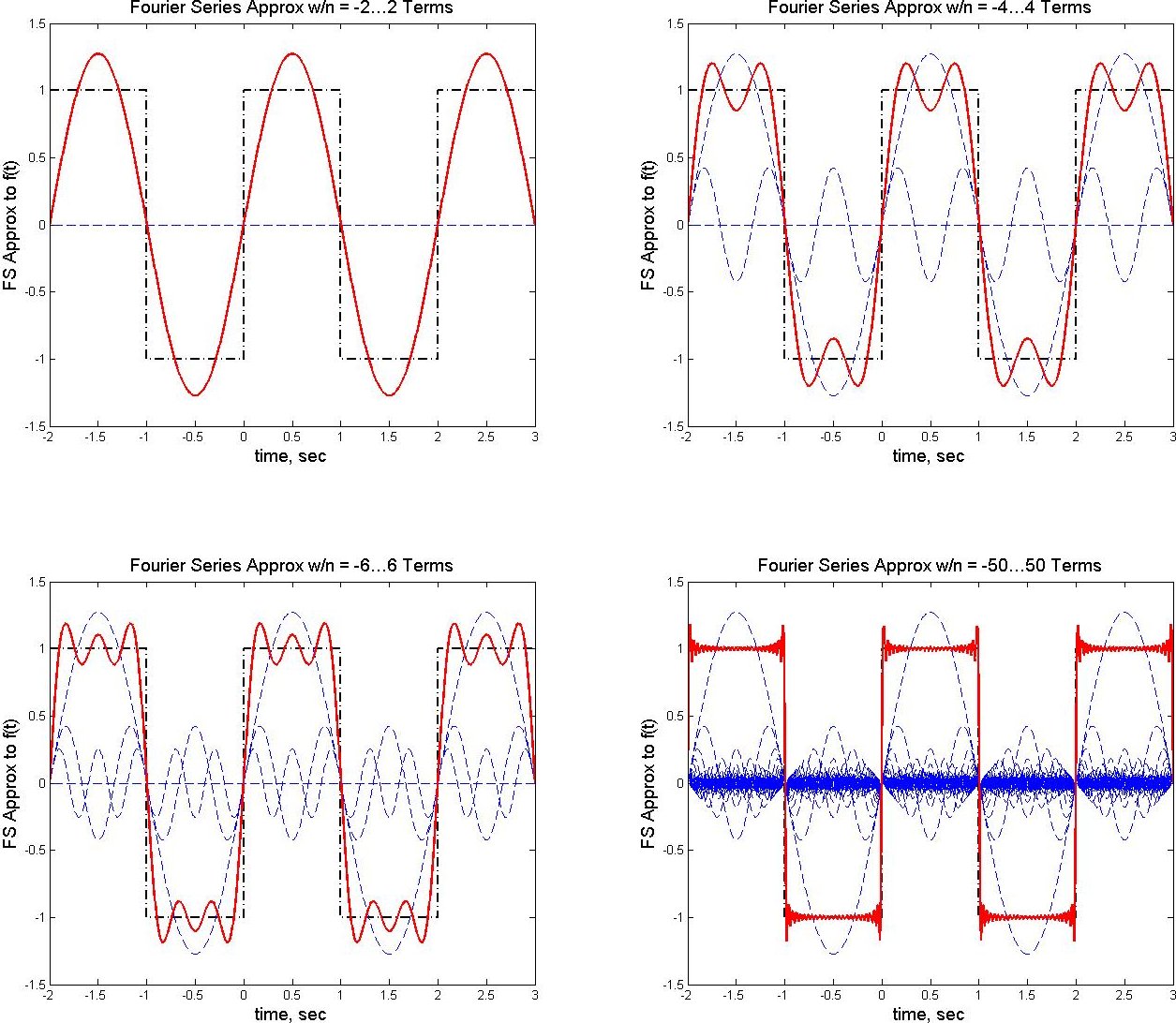
        % representation of a square wave.
        
        clear; clc; close all; % clear memory and command window, close all figures
        
        t = linspace(-2,3,1000); % times over which to plot FS
        
        N = [2, 4, 6, 50]; % upper limit (N) and lower limit (-N) for n in summation
        
        figure(1); % open figure in which to plot
        
        % Build square wave using increasing number of terms
        for in = 1:4, % loop over four different limits (in N) of Fourier Series
          f = zeros(1,length(t)); % initialize summation to c0
          subplot(2,2,in); % open one of four subplots
          % brute force original square wave
          plot([-2, -1, -1,  0, 0, 1,  1,  2, 2, 3],...
               [ 1,  1, -1, -1, 1, 1, -1, -1, 1, 1],'k-.','LineWidth',2);
          hold on;
          for n = 1:1:N(in), % loop over different lengths of FS
            termpos = ((1 - cos( n*pi))/( j*n*pi))*exp( j*n*pi*t); %compute +n term
            termneg = ((1 - cos(-n*pi))/(-j*n*pi))*exp(-j*n*pi*t); %compute -n term
            terms   = termpos + termneg; % add complex conjugate terms to get real terms
            f       = f + terms; % add real terms to series
            plot(t,terms,'b--','LineWidth',1); % plot real terms (harmonics)
          end
          plot(t,f,'r-','LineWidth',2); % plot FS
          hold off;
          xlabel('time, sec','FontSize',14); ylabel('FS Approx to f(t)','FontSize',14);
          title(['Fourier Series Approx w/n = ',num2str(-N(in)),'\ldots', num2str(N(in)),' Terms'],'FontSize',14);
        end
      

Figures/Plots Generated: