Plotting Frequency Responses using Matlab

(Amplitude/Magnitude in dB, Frequency on Logarithmic Axes)

M-file:

                %% EE 212 - FrequencyResponseExample2.m
                %
                % Description:  M-file showing how to plot frequency responses (magnitude
                % in dB and phase angle, both versus angular frequency on a logarithmic axis)
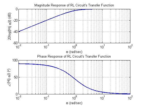
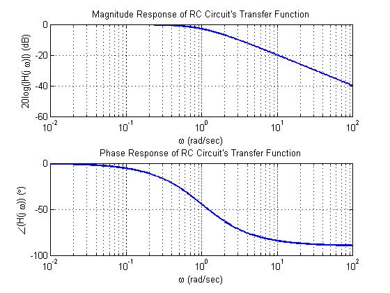
                % for three circuits.  The RL circuit is a high-pass filter, the RC
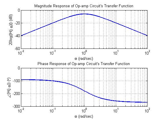
                % circuit is a low-pass filter, and the op-amp circuit with two capacitors
                % is a band-pass filter.
                %
                
                %% Clear memory; clear command window; close all existing figures
                clear; clc; close all;
                
                %% RL circuit's (high-pass) frequency response on logarithmic omega-axes
                % vector of 250 logarithmically-spaced frequencies between 10^-2 and 10^2
                w = logspace(-2,2,250);
                R = 1; L = 1;               % values of resistor and inductor
                H = (j*w*L)./(R + j*w*L);   % (complex) transfer function
                figure(1);                  % open first figure
                % plot magnitude response in top half of first figure, and label
                subplot(2,1,1);
                semilogx(w, 20*log10(abs(H)), 'linewidth', 2);
                grid;
                xlabel('\omega (rad/sec)'); ylabel('20log(|H(j \omega)|) (dB)')
                title('Magnitude Response of RL Circuit''s Transfer Function');
                % plot phase response (using degrees) in bottom half of first figure, and label
                subplot(2,1,2);
                semilogx(w, unwrap(angle(H))*180/pi, 'linewidth', 2);
                grid;
                xlabel('\omega (rad/sec)'); ylabel('\angle(H(j \omega)) (\circ)')
                title('Phase Response of RL Circuit''s Transfer Function');
                
                %% RC circuit's (low-pass) frequency response on logarithmic omega-axes
                % vector of 250 logarithmically-spaced frequencies between 10^-2 and 10^2
                w = logspace(-2,2,250);
                R = 1; C = 1;               % values of resistor and capacitor
                H = 1./(j*w*R*C + 1);       % (complex) transfer function
                figure(2);                  % open second figure
                % plot magnitude response in top half of first figure, and label
                subplot(2,1,1);
                semilogx(w, 20*log10(abs(H)), 'linewidth', 2);
                grid;
                xlabel('\omega (rad/sec)'); ylabel('20log(|H(j \omega)|) (dB)')
                title('Magnitude Response of RC Circuit''s Transfer Function');
                % plot phase response (using degrees) in bottom half of first figure, and label
                subplot(2,1,2);
                semilogx(w, unwrap(angle(H))*180/pi, 'linewidth', 2);
                grid;
                xlabel('\omega (rad/sec)'); ylabel('\angle(H(j \omega)) (\circ)')
                title('Phase Response of RC Circuit''s Transfer Function');
                
                %% Op-amp circuit's (band-pass) frequency response on logarithmic omega-axes
                % vector of 250 logarithmically-spaced frequencies between 10^-2 and 10^2
                w = logspace(-2,2,250);
                H = (-j*w)./(1 + j*w).^2;   % (complex) transfer function
                figure(3);                  % open third figure
                % plot magnitude response in top half of first figure, and label
                subplot(2,1,1);
                semilogx(w, 20*log10(abs(H)), 'linewidth', 2);
                grid;
                xlabel('\omega (rad/sec)'); ylabel('20log(|H(j \omega)|) (dB)')
                title('Magnitude Response of Op-amp Circuit''s Transfer Function');
                % plot phase response (using degrees) in bottom half of first figure, and label
                subplot(2,1,2);
                semilogx(w, unwrap(angle(H))*180/pi, 'linewidth', 2);
                grid;
                xlabel('\omega (rad/sec)'); ylabel('\angle(H(j \omega)) (\circ)')
                title('Phase Response of Op-amp Circuit''s Transfer Function');
            

Figures/Plots Generated: