Plotting Frequency Responses using Matlab

(Amplitude/Magnitude in dB, Frequency on Logarithmic Axes)

M-file:

                %% EE 212 - FrequencyResponseExample3.m
                %
                % Description:  M-file showing Bode Plots (via Matlab) for in-class examples.
                %
                
                %% Clear memory; clear command window; close all existing figures
                clear; clc; close all;
                
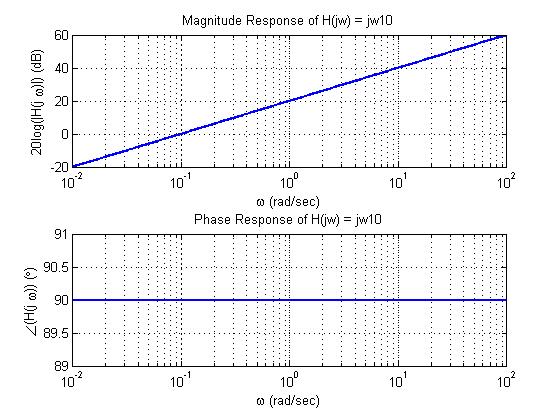
                %% H(jw) = jw10
                % vector of 250 logarithmically-spaced frequencies between 10^-2 and 10^2
                w = logspace(-2,2,250);
                H = j*w*10;                 % (complex) transfer function
                figure(1);                  % open first figure
                % plot magnitude response in top half of first figure, and label
                subplot(2,1,1);
                semilogx(w, 20*log10(abs(H)), 'linewidth', 2);
                grid;
                xlabel('\omega (rad/sec)'); ylabel('20log(|H(j \omega)|) (dB)')
                title('Magnitude Response of H(jw) = jw10');
                % plot phase response (using degrees) in bottom half of first figure, and label
                subplot(2,1,2);
                semilogx(w, unwrap(angle(H))*180/pi, 'linewidth', 2);
                grid;
                xlabel('\omega (rad/sec)'); ylabel('\angle(H(j \omega)) (\circ)')
                title('Phase Response of H(jw) = jw10');
                
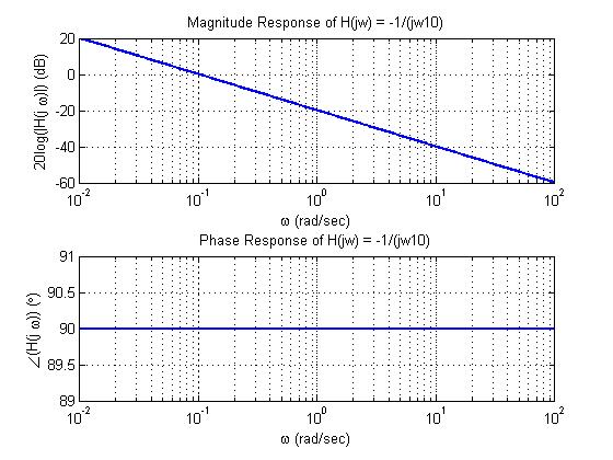
                %% H(jw) = -1/(jw10)
                % vector of 250 logarithmically-spaced frequencies between 10^-2 and 10^2
                w = logspace(-2,2,250);
                H = -1./(j*w*10);           % (complex) transfer function
                figure(2);                  % open second figure
                % plot magnitude response in top half of first figure, and label
                subplot(2,1,1);
                semilogx(w, 20*log10(abs(H)), 'linewidth', 2);
                grid;
                xlabel('\omega (rad/sec)'); ylabel('20log(|H(j \omega)|) (dB)')
                title('Magnitude Response of H(jw) = -1/(jw10)');
                % plot phase response (using degrees) in bottom half of first figure, and label
                subplot(2,1,2);
                semilogx(w, unwrap(angle(H))*180/pi, 'linewidth', 2);
                grid;
                xlabel('\omega (rad/sec)'); ylabel('\angle(H(j \omega)) (\circ)')
                title('Phase Response of H(jw) = -1/(jw10)');
                
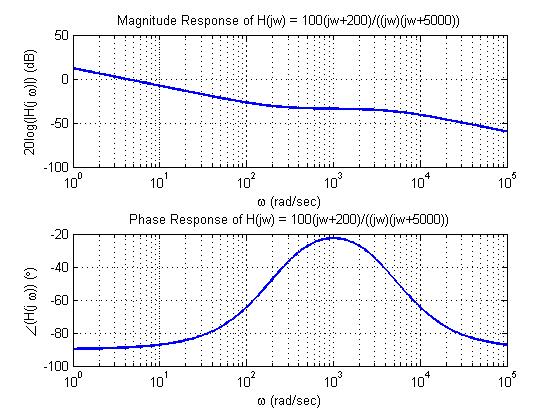
                %% H(jw) = 100(jw+200)/((jw)(jw+5000))
                % vector of 250 logarithmically-spaced frequencies between 10^0 and 10^5
                w = logspace(0,5,250);
                H = 100*(j*w+200)./((j*w).*(j*w+5000)); % (complex) transfer function
                figure(3);                              % open third figure
                % plot magnitude response in top half of first figure, and label
                subplot(2,1,1);
                semilogx(w, 20*log10(abs(H)), 'linewidth', 2);
                grid;
                xlabel('\omega (rad/sec)'); ylabel('20log(|H(j \omega)|) (dB)')
                title('Magnitude Response of H(jw) = 100(jw+200)/((jw)(jw+5000))');
                % plot phase response (using degrees) in bottom half of first figure, and label
                subplot(2,1,2);
                semilogx(w, unwrap(angle(H))*180/pi, 'linewidth', 2);
                grid;
                xlabel('\omega (rad/sec)'); ylabel('\angle(H(j \omega)) (\circ)')
                title('Phase Response of H(jw) = 100(jw+200)/((jw)(jw+5000))');
            

Figures/Plots Generated: