EE 212L: Op-Amp Differentiators and Integrators
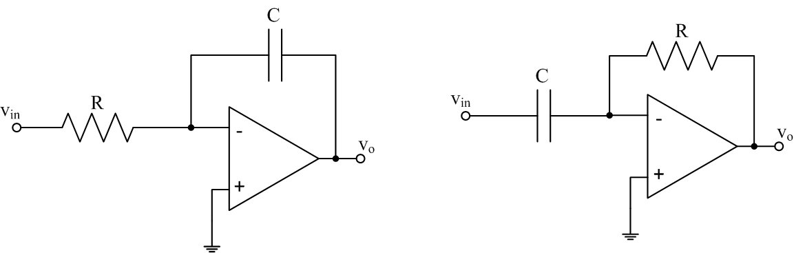
Objective: Op-amp circuits are often designed and implemented for signal differentiation and integration. Until recently (before computer-based control), control algorithms (such as PID) containing differentials and integrals were implemented in discrete circuit components. Differentiation is also useful for obtaining velocity measurements from a signal representing a position or determining a signal's frequency (recall the amplitude of the time derivative of a sinusoid is scaled by its frequency). Figure 1 below shows an ideal op-amp integrator and differentiator with input-output relationships that are theoretically correct, but have practical implementation issues discussed below. In this lab, practically realizable differentiators and integrators will be built using op-amps, resistors and capacitors.
Pre-lab:
- Use time-based methods (i.e., differential and integral v-i relationships) to find the input-output voltage relationships for the ideal op-amp integrator and differentiator shown in Figure 1 of the lab. These equations should confirm that one circuit integrates vin and the other differentiates vin.
- Use sinusoidal steady-state (AC) analysis to show the phasor input-output voltage relationship (transfer function) is H(jω) = Vo/Vin = -jωRC for the ideal differentiator and H(jω) = Vo/Vin = -1/(jωRC) for the ideal integrator.
- Figure 2 of the lab shows a practical implementation of a differentiator. Derive the transfer function H(jω) = Vo/Vin for this circuit. For what frequencies does the circuit act as a differentiator? What effective operation is performed by the circuit at high frequencies?
- Figure 3 of the lab shows a practical implementation of an integrator. Derive the transfer function H(jω)=Vo/Vin for this circuit. For what frequencies does this circuit act as an integrator? How does the circuit respond to low frequencies?
Laboratory Procedure:
- The Differentiator
- The ideal differentiator is inherently unstable in practice
due to the presence of some high frequency noise in every
electronic system. An ideal differentiator would amplify this
small noise. For instance, if vnoise =
Asin(ωt) is differentiated, the output would
be vout = Aωcos(ωt). Even if A =
1μV, when ω = 2π(10MHz), vout would have
an amplitude of 63V! To circumvent this problem, it is
traditional to include a series resistor at the input and a
parallel capacitor across the feedback resistor as shown in
Figure 2, converting the differentiator to an integrator at high
frequencies for filtering.
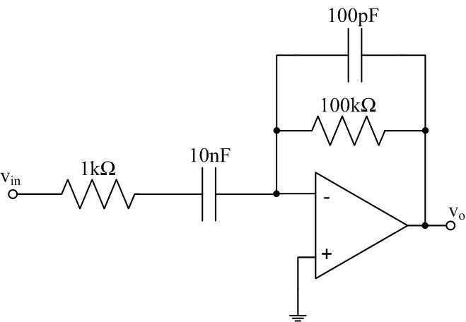
Figure 2: Improved differentiator circuit for practical implementation
- Wire up the practical op-amp differentiator shown in Figure 2 using your op-amp of choice (e.g., 741 or 356).
- Drive it (via vin(t)) with a 1kHz sine wave, a 1kHz square wave, and a 1kHz triangle wave. For each input signal, sketch the input and output waveforms.
- Are the output waveforms and their amplitudes what you would expect, i.e., does the circuit differentiate the input signal?
- The ideal differentiator is inherently unstable in practice
due to the presence of some high frequency noise in every
electronic system. An ideal differentiator would amplify this
small noise. For instance, if vnoise =
Asin(ωt) is differentiated, the output would
be vout = Aωcos(ωt). Even if A =
1μV, when ω = 2π(10MHz), vout would have
an amplitude of 63V! To circumvent this problem, it is
traditional to include a series resistor at the input and a
parallel capacitor across the feedback resistor as shown in
Figure 2, converting the differentiator to an integrator at high
frequencies for filtering.
- The Integrator
- Op-amps allow you to make nearly perfect integrators such as
the practical integrator shown in Figure 3. The circuit
incorporates a large resistor in parallel with the feedback
capacitor. This is necessary because real op-amps have a small
current flowing at their input terminals called the "bias
current". This current is typically a few nanoamps, and is
neglected in many circuits where the currents of interest are in
the microamp to milliamp range. However, if you apply a nanoamp
current to a 0.1μF capacitor, it won't take long until it
charges and becomes effectively an open circuit not allowing any
current to flow! The feedback resistor gives a path for the bias
current to flow. The effect of the resistor on the response is
negligible at all but the lowest frequencies.
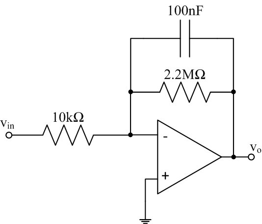
Figure 3: Improved integrator circuit for practical implementation
- Wire up the practical op-amp integrator shown in Figure 3.
- Drive the input (via vin(t)) with a 500Hz square wave of 2 V p-p amplitude. Sketch the input and output waveforms.
- Does it appear that the input been integrated?
- Calculate the expected output waveform via analytical integration using the circuit component values, and compare to the experimental waveform.
- Does the amplitude of the output waveform agree with what it should be from the circuit values?
- Repeat (test your integrator) using a sine wave and a triangle wave.
- Op-amps allow you to make nearly perfect integrators such as
the practical integrator shown in Figure 3. The circuit
incorporates a large resistor in parallel with the feedback
capacitor. This is necessary because real op-amps have a small
current flowing at their input terminals called the "bias
current". This current is typically a few nanoamps, and is
neglected in many circuits where the currents of interest are in
the microamp to milliamp range. However, if you apply a nanoamp
current to a 0.1μF capacitor, it won't take long until it
charges and becomes effectively an open circuit not allowing any
current to flow! The feedback resistor gives a path for the bias
current to flow. The effect of the resistor on the response is
negligible at all but the lowest frequencies.
Revised MAR2015