EE 212L: RC Time Constant, Square-waves and Probe Compensation
Objective: The purpose of this lab is to measure square-wave responses of an RC circuit to gain a better understanding of first-order circuits and time constants, and learn how to calibrate an oscilloscope probe.
Pre-lab: Consider the RC circuit of Figure 5 shown below.
- What is the theoretical time constant τ ("tau") for the circuit?
- Sketch one period of the output voltage vo on
top of the input square-wave shown in Figure 1 when the input's
period T is specified as
- T = 10 τ
- T = 1 τ
- T = τ / 10
Figure 1: Square-wave input voltage vi
- Calculate the relationship between the 10% to 90% rise time (as
shown in Figure 2 below), and the time constant τ for the
circuit's step response. Hint: you'll need to solve for the step
response of the circuit.
Figure 2: Rise time for first-order step response
Laboratory Procedure:
- Calibration and probe settings for the oscilloscope. A probe and
its cable have an inherent resistance and capacitance that make the
probe's behavior between the input (signal we wish to measure) and
output (connection to oscilloscope) vary as a function of the signal's
frequency. To enable more accurate measurements at low frequencies
(say under 100kHz) probes come with an adjustable capacitor that can
be used to match the inherent time constant of the probe and cable. It
is good practice to calibrate your probe each time before use to
ensure meaningful measurements.
- Display the 1kHz square-wave from the probe comp output
of your oscilloscope as shown in Figure 3. Adjust the trigger,
vertical scale and horizontal scale as needed to obtain a good
view of a stable waveform.
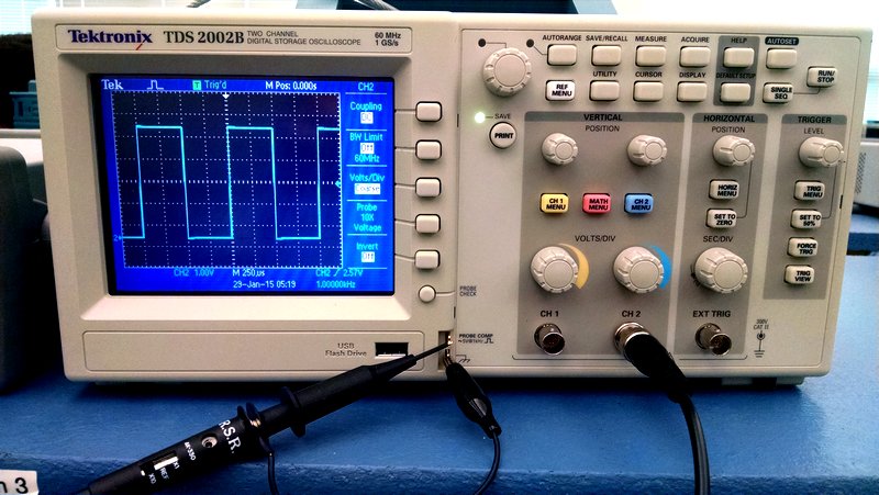
Figure 3: Probe connection to oscilloscope's PROBE COMP output
- Measure the amplitude of the waveform with the scope probe in both the 1X and 10X positions. Note whether you adjusted the corresponding settings on the oscilloscope.
- Compensate the probe in the 10X position to by
adjusting a small screw in the probe until the square wave is
shown properly. Examples of measurements from under-, over- and
properly compensated probes are shown in Figure 4 below.
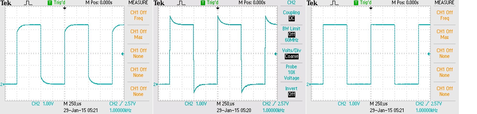
Figure 4: Display of square wave when probe is under-compensated (left), over-compensated (center) and properly compensated (right).
Draw the shapes of your measured square wave when the probe is under-compensated and over-compensated. - Adjust your probe to be properly compensated before continuing.
- Why would one choose to use a 10X probe versus one without the built-in attenuation? (There are at least 3 possible reasons.)
- Display the 1kHz square-wave from the probe comp output
of your oscilloscope as shown in Figure 3. Adjust the trigger,
vertical scale and horizontal scale as needed to obtain a good
view of a stable waveform.
- Observe square waveforms using the oscilloscope and investigate
effects of AC versus DC coupling.
- Set the frequency of your function generator to approximately 10 Hz and the waveform to a 5V peak-to-peak square-wave, and then a 5V peak-to-peak triangle-wave. Set up the oscilloscope to view these waveforms.
- Note and sketch differences for the two waveforms when the scope input is AC or DC coupled. Explain why the signal is degraded on AC coupling? Use DC coupling for the rest of this lab.
- Measure rise time of a function generator square-wave.
- Set the frequency of a 5V peak-to-peak square-wave to 1MHz on the function generator and measure the rise-time of the square-wave (i.e., the time it takes to go from 10% to 90% of its final value while rising) using the oscilloscope by expanding the time base.
- View and investigate RC circuit step responses.
- Construct the RC circuit shown in Figure 5 below on your
breadboard and use your function generator to provide a 1V
square-wave input vi for different periods (T = 10
τ, τ and τ / 10). Display both the input
vi and output vo on the
o-scope using Channels 1 and 2. Trigger on the rising edge of the
input. Use the 10X probe and interpret your measurements
accordingly.
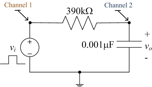
Figure 5: Series RC circuit
- Sketch the output waveforms over a single period for signal input periods of T = 10 τ, τ and τ / 10. Label your axes. Explain the form of these plots and compare to your theoretical waveforms done in the prelab. For which pulse length does the output most resemble the input?
- For the input period T = 10 τ, the initial part of the waveform is equivalent to the step response of the circuit. Use the relationship obtained in the prelab to determine the time constant of this circuit by measuring the 10% to 90% rise time. Compare with the theoretical time constant.
- Repeat the previous two parts with the resistor and capacitor
interchanged. Note this circuit setup can be thought of as
similar to the AC coupling studied in part 1. Sketch the
circuit, sketch the input and output waveforms as the input
period is varied, and answer the following questions:
- For which pulse length does the output most resemble the input?
- Why does the output waveform go above the maximum and below the minimum values of the square-wave?
- Why isn't the output amplitude constant?
- Construct the RC circuit shown in Figure 5 below on your
breadboard and use your function generator to provide a 1V
square-wave input vi for different periods (T = 10
τ, τ and τ / 10). Display both the input
vi and output vo on the
o-scope using Channels 1 and 2. Trigger on the rising edge of the
input. Use the 10X probe and interpret your measurements
accordingly.
- Measure the inductor provided in your kit. You'll need this value for next week's lab.
Revised JAN2015