EE 212L: Step Responses of RL and RLC Circuits
Objective: The purpose of this lab is to study the first-order step response of a series RL circuit and the underdamped, second-order step response of a series RLC circuit. Key aspects of interest will be creation of a step function with the function generator, verification of steady-state (DC) behavior, and calculation of common metrics associated with step responses.
Pre-lab:
- Determine and plot the step response (i(t) for vi(t) = u(t)) of the circuit shown in Figure 1 below. Use R = 150 Ω and the value of your inductor measured at the end of last week's lab. Fill in the "predicted column" of the table of metrics below with values obtained from the calculated step response.
- In part 2 of the lab, the series RLC circuit shown in Figure 3 is desired
to have an underdamped step response with specified attributes.
Choose R, L, and C so that the specifications given are met. Determine and plot the step response
(v(t) for vi(t) = u(t)). Fill in the second table of metrics
(predicted column) with values obtained from your calculated step response.
- Here is a Matlab m-file to use as a starting point for plotting the solution to this problem. Also, if you look carefully, you will see a way of checking your answer.
Laboratory Procedure:
-
Use function generator to create a square wave that will used
as unit step input for the two circuits below. Choose a period
for the square wave greater than ten time constants (10 τ)
for the circuit in Figure 1 with R = 150 Ω and L the value
of your inductor measured at the end of last week's lab. The
square wave should transition between 0V and 1V. Items to keep in mind:
- The function generator has an output resistance of 50 Ω which may be significant if the resistance in your circuit is small. Be careful with the function generator's setting related to load resistance as it gives a choice of 50 Ω or infinite which only changes its displayed values (not the actual output) for amplitude and DC offset. Infinite is likely the better setting as the amplitude and DC offset match typical definitions.
- By default, the function generator centers waveforms vertically about zero, so to shift a waveform up (say between 0V and 1V) a DC offset will be needed.
-
Construct the circuit shown in Figure 1 below. Use a R = 150 Ω
resistor and the inductor in your kit (measured last week).
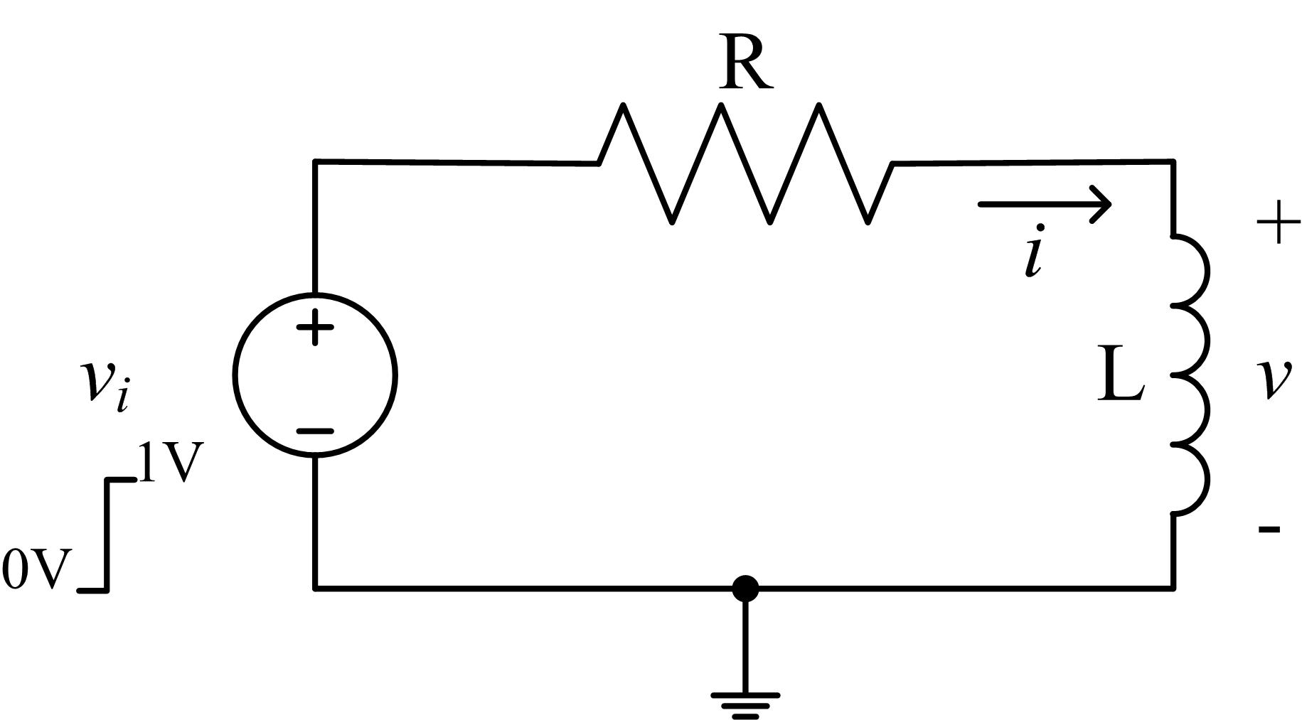
Figure 1: Series RL circuit
- Generate a step input, vi(t) = u(t), by using a 1V square wave (use the dc offset to achieve the desired 0V to 1V transitions) with a period sufficiently long (i.e., at least 10τ) so that the output reaches steady-state before the input transitions. When measured on the oscilloscope, does the square wave span 0V to 1V? If not, note why, and correct it.
- Sketch the response and record the specified step response metrics of Figure 2 in a table similar to the following. The math function on the oscilloscope may be a useful feature when trying to display current. Compare the predicted and measured values.
Metric Predicted Measured Initial value, i(0) Final (steady-state, DC) value, iss = i(∞) 10% - 90% rise-time, Tr Settling time (to within 5% of iss), Ts Percent overshoot, 100% × (peak value - iss) / iss Time constant, τ 
Figure 2: Common metrics associated with step responses
- Construct the circuit shown in Figure 3 below.
- Determine values of R, L, and C for the circuit shown in Figure 3 so that
the step response is underdamped (exponentially-damped sinusoid)
with an exponential decay governed
by an α of 105 (i.e. the damped sinusoidal response goes
to e-1 of its final value in 10 μseconds) and a frequency
of 1MHz. Use the 0.47mH inductor in your parts kit for L.
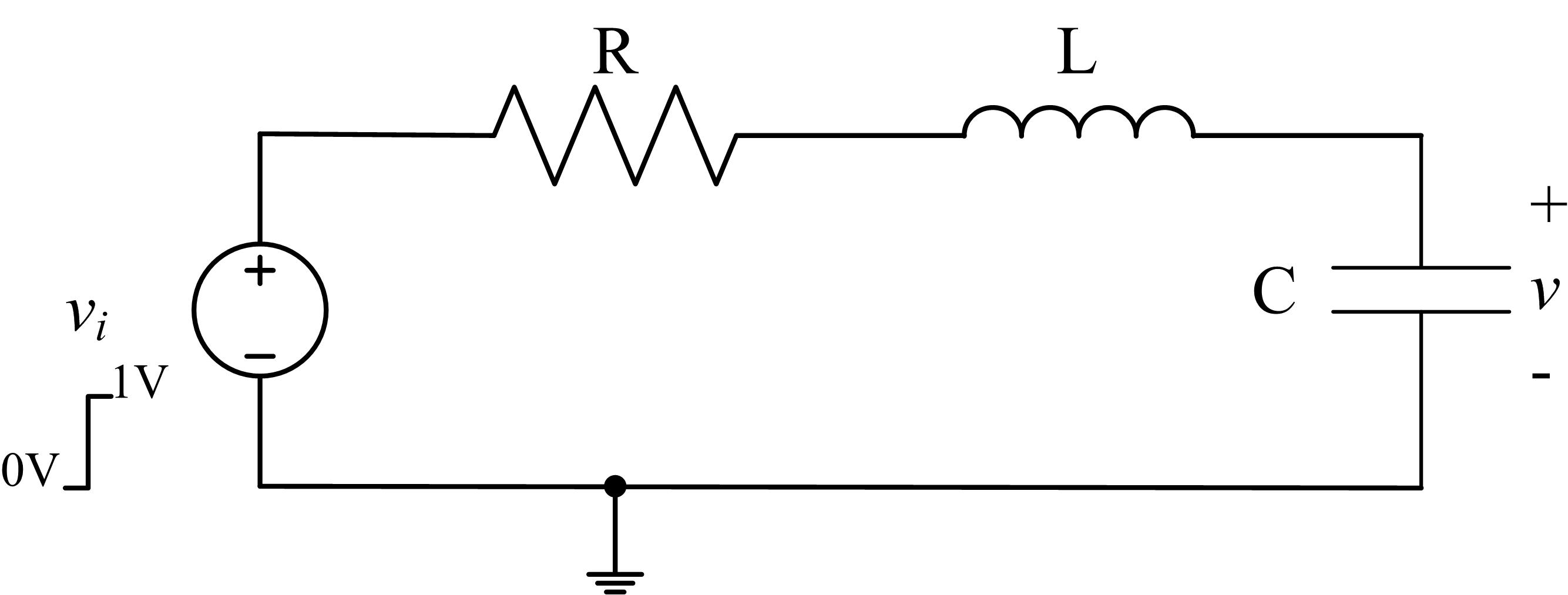
Figure 3: Series RLC circuits
- Use the function generator for the unit step input, and observe the step response for v. Compare the theoretical response with your measurements using a table similar to that shown below. For this underdamped RLC circuit, the response should have the form v(t) = vss (1 - e-αtcos(ωt + θ))u(t).
-
Fill in the table below with metrics measured with the help of the
oscilloscope.
Metric Predicted Measured Initial value, v(0) Final (steady-state, DC) value, vss = v(∞) 10% - 90% rise-time, Tr Settling time (to within 5% of vss), Ts Percent overshoot, 100% × (peak value - vss) / vss Exponent, α Frequency, ω
- Determine values of R, L, and C for the circuit shown in Figure 3 so that
the step response is underdamped (exponentially-damped sinusoid)
with an exponential decay governed
by an α of 105 (i.e. the damped sinusoidal response goes
to e-1 of its final value in 10 μseconds) and a frequency
of 1MHz. Use the 0.47mH inductor in your parts kit for L.
Revised FEB2015