EE341.01: MATLAB M-FILE FOR PLOTTING TRUNCATED FOURIER SERIES

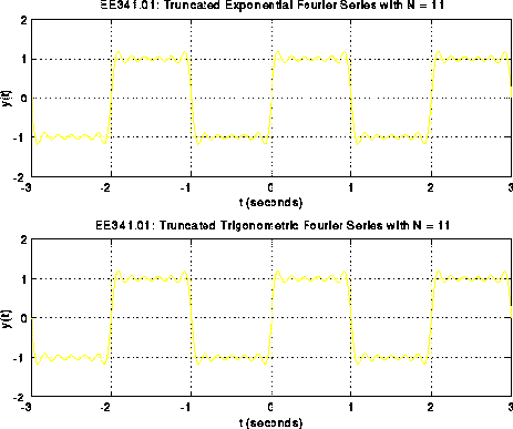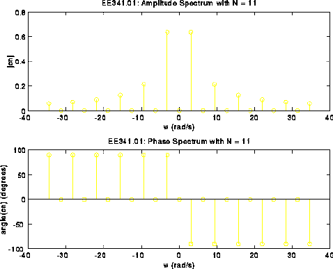
This example shows a MATLAB M-file for plotting the truncated Fourier Series of a square wave. The amplitude and phase spectrums are also plotted.

%
% Filename: example8.m
%
% Description: This M-file plots the truncated Fourier Series
%              for a square wave as well as its amplitude
%              spectrum.

clear;                             % clear all variables
clf;                               % clear all figures

N = 11;                            % summation limit (use N odd)
wo = pi;                           % fundamental frequency (rad/s)
c0 = 0;                            % dc bias
t = -3:0.01:3;                     % declare time values

figure(1)                          % put first two plots on figure 1

% Compute yce, the Fourier Series in complex exponential form

yce = c0*ones(size(t));            % initialize yce to c0

for n = -N:2:N,                    % loop over series index n
  cn = 2/(j*n*wo);                 % Fourier Series Coefficient
  yce = yce + cn*exp(j*n*wo*t);    % Fourier Series computation
end

subplot(2,1,1)
plot([-3 -2 -2 -1 -1  0 0 1  1  2 2 3],...    % plot original y(t)
     [-1 -1  1  1 -1 -1 1 1 -1 -1 1 1], ':');
hold;
plot(t,yce);
grid;
xlabel('t (seconds)')
ylabel('y(t)');
ttle = ['EE341.01: Truncated Exponential Fourier Series with N = ',...
         num2str(N)];
title(ttle);
hold

% Compute yt, the Fourier Series in trigonometric form

yt = c0*ones(size(t));             % initialize yce to c0

for n = 1:2:N,                     % loop over series index n
  cn = 2/(j*n*wo);                 % Fourier Series Coefficient
  yt = yt + 2*abs(cn)*cos(n*wo*t+angle(cn));  % Fourier Series computation
end

subplot(2,1,2)
plot([-3 -2 -2 -1 -1  0 0 1  1  2 2 3],...    % plot original y(t)
     [-1 -1  1  1 -1 -1 1 1 -1 -1 1 1], ':');
hold;
plot(t,yt);
grid;
xlabel('t (seconds)')
ylabel('y(t)');
ttle = ['EE341.01: Truncated Trigonometric Fourier Series with N = ',...
         num2str(N)];
title(ttle);
hold

% Draw the amplitude spectrum from exponential Fourier Series

figure(2)                          % put next plots on figure 2

subplot(2,1,1)
stem(0,c0);                        % plot c0 at nwo = 0

hold
for n = -N:2:N,                    % loop over series index n
  cn = 2/(j*n*wo);                 % Fourier Series Coefficient
  stem(n*wo,abs(cn))               % plot |cn| vs nwo
end
for n = -N+1:2:N-1,                % loop over even series index n 
  cn = 0;                          % Fourier Series Coefficient
  stem(n*wo,abs(cn)*180/pi);       % plot |cn| vs nwo
end

xlabel('w (rad/s)')
ylabel('|cn|')
ttle = ['EE341.01: Amplitude Spectrum with N = ',num2str(N)];
title(ttle);
hold

% Draw the phase spectrum from exponential Fourier Series

subplot(2,1,2)
stem(0,angle(c0)*180/pi);                 % plot angle of c0 at nwo = 0

hold
for n = -N:2:N,                    % loop over odd series index n 
  cn = 2/(j*n*wo);                 % Fourier Series Coefficient
  stem(n*wo,angle(cn)*180/pi);     % plot |cn| vs nwo
end
for n = -N+1:2:N-1,                % loop over even series index n 
  cn = 0;                          % Fourier Series Coefficient
  stem(n*wo,angle(cn)*180/pi);     % plot |cn| vs nwo
end

xlabel('w (rad/s)')
ylabel('angle(cn) (degrees)')
ttle = ['EE341.01: Phase Spectrum with N = ',num2str(N)];
title(ttle);
hold