EE341 EXAMPLE 5: PLOTTING TRUNCATED FOURIER SERIES REPRESENTATION AND SPECTRA OF A SIGNAL

%
% Filename: example5.m
%
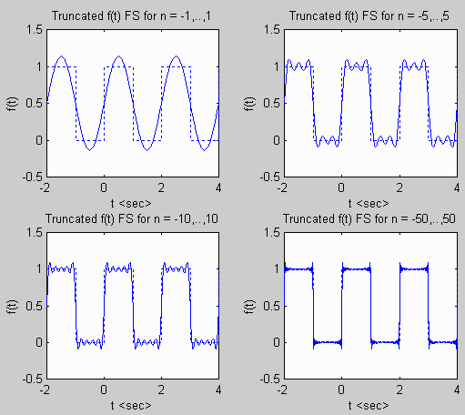
% Description: m-file to compute and plot the truncated Fourier
%              Series representation of a square wave.
%

% *** Plot truncatated FS for various numbers of terms. ***
clear;                                      % clear matlab's memory
figure(1); clf;	                            % open and clear figure 1

To = 2; wo = 2*pi/To;                       % fundamental period and frequency

D0 = 0.5;                                   % signal offset

t = -2:0.01:4;		                    % time over which we'll plot signal

N = [1 5 10 50];                            % +/- values at which we'll truncate FS

for i = 1:4,				    % compute truncated FS for above N values
   
   f = D0*ones(size(t));                    % start out with DC bias term
   
   for n = -N(i):-1,                        % loop over negative n
      Dn = (1 - exp(-j*n*pi))/(j*2*pi*n);   % Fourier coefficient
      f = f + real(Dn*exp(j*n*wo*t));       % add FS terms
   end;
   
   for n = 1:N(i),                          % loop over positive n
      Dn = (1 - exp(-j*n*pi))/(j*2*pi*n);   % Fourier coefficient
      f = f + real(Dn*exp(j*n*wo*t));       % add FS terms
   end;
   
   subplot(2,2,i);                          % plot truncated FS representation of f(t)
   plot(t,f);                               % and actual signal
   hold on;
   plot([-2 -1 -1 0 0 1 1 2 2 3 3 4 4],[1 1 0 0 1 1 0 0 1 1 0 0 1],':');
   hold off;
   xlabel('t ');
   ylabel('f(t)');
   titlevec = ['Truncated f(t) FS for n = ' num2str(-N(i)),',..,',num2str(N(i))];
   title(titlevec);
   
end;

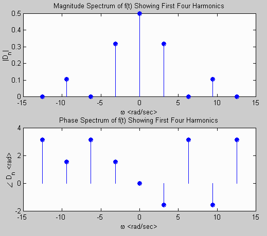
% *** Plot exponential magnitude and phase spectra for 1st 4 harmonics
clear;						% clear matlab's memory
figure(2); clf;					% open and clear figure 2

To = 2; wo = 2*pi/To;			        % fundamental period and frequency

D0 = 0.5;					% signal offset, 0 frequency term

i = 1;						% vector index to help store Dn and w

for n = -4:-1,					% loop over negative n
   Dn(i) = (1 - exp(-j*n*pi))/(j*2*pi*n);	% Compute & store fourier coef.
   w(i) = n*wo;					% store associated frequency
	i = i + 1;				% increment vector index   
end;

Dn(i) = D0; w(i) = 0;                           % store 0 frequency terms							
i = i + 1;					% increment vector index

for n = 1:4,					% loop over positive n
   Dn(i) = (1 - exp(-j*n*pi))/(j*2*pi*n);	% Compute & store Fourier coef.
   w(i) = n*wo;					% store associated frequency
   i = i + 1;					% increment vector index;
end;
   
subplot(2,1,1);					% plot magnitude spectrum of f(t)
stem(w,abs(Dn),'filled');
xlabel('\omega ');
ylabel('|D_n|');
title('Magnitude Spectrum of f(t) Showing First Four Harmonics');

subplot(2,1,2);					% plot phase spectrum of f(t)
stem(w,angle(Dn),'filled');
xlabel('\omega ');
ylabel('\angle D_n ');
title('Phase Spectrum of f(t) Showing First Four Harmonics');