%
% Filename: example7.m
%
% Description: M-file for displaying RLC circuit response to
% periodic input.
%
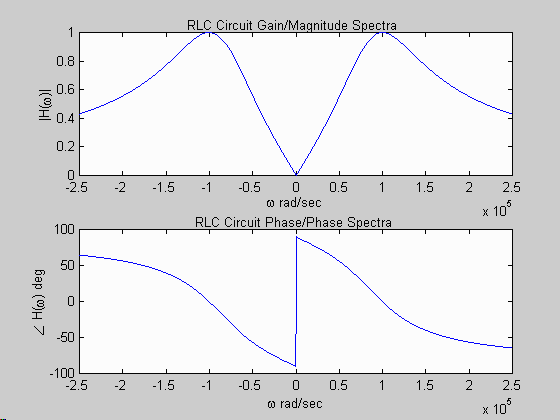
%** System Spectra **%
clear; % clear matlab memory
R = 100; L = 1e-3; C = 100e-9; % define circuit parameters
w = -250000:2:250000; % frequency values for spectra
H = (R/L)*j*w./((j*w).^2 + (R/L)*j*w + 1/(L*C)); % system TF
figure(1); clf; % open and clear figure 1
subplot(2,1,1); plot(w,abs(H)); % plot magnitude spectrum
xlabel('\omega rad/sec'); ylabel('|H(\omega)|');
title('RLC Circuit Gain/Magnitude Spectra');
subplot(2,1,2); plot(w,angle(H)*180/pi); % plot phase spectrum
xlabel('\omega rad/sec'); ylabel('\angle {H(\omega) deg}');
title('RLC Circuit Phase/Phase Spectra');
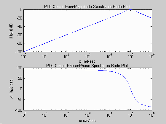
%** System Specta as Bode Plots **%
figure(2); clf; % open and clear figure 2
w = 1:2:1e6; % frequency values for spectra
H = (R/L)*j*w./((j*w).^2 + (R/L)*j*w + 1/(L*C)); % system TF
subplot(2,1,1); semilogx(w,20*log10(abs(H))); % plot magnitude spectrum
xlabel('\omega rad/sec'); ylabel('|H(\omega)| dB');
title('RLC Circuit Gain/Magnitude Spectra as Bode Plot');
subplot(2,1,2); semilogx(w,angle(H)*180/pi); % plot phase spectrum
xlabel('\omega rad/sec'); ylabel('\angle {H(\omega)} deg');
title('RLC Circuit Phase/Phase Spectra as Bode Plot');
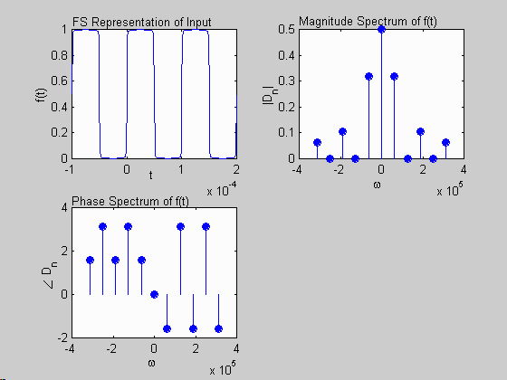
%** Input FS Representation **%
figure(3); clf; % open and clear figure 3
N = 100; % +/- number of FS terms taken
To = 100e-6; wo = 2*pi/To; % fundamental period and frequency
D0 = 0.5; % signal offset
t = -100e-6:1e-6:200e-6; % time over which we'll plot signal
f = D0*ones(size(t)); % start out with DC bias term
for n = -N:-1, % loop over negative n
Dn = (1-exp(-j*pi*n))./(j*2*pi*n); % Fourier coefficient
f = f + real(Dn*exp(j*n*wo*t)); % add FS terms
end;
for n = 1:N, % loop over positive n
Dn = (1-exp(-j*pi*n))./(j*2*pi*n); % Fourier coefficient
f = f + real(Dn*exp(j*n*wo*t)); % add FS terms
end;
subplot(2,2,1); plot(t,f); % plot truncated f(t) FS
xlabel('t '); ylabel('f(t)');
title('FS Representation of Input');
%** Input exponential magnitude and phase spectra for 1st 5 harmonics **%
i = 1; % vector index to help store Dn and w
w = 0; Dn = 0; % reinitialize FS variables
for n = -5:-1, % loop over negative n
Dn(i) = (1-exp(-j*pi*n))./(j*2*pi*n); % Fourier coefficient
w(i) = n*wo; % store associated frequency
i = i + 1; % increment vector index
end;
Dn(i) = D0; w(i) = 0; % store 0 frequency terms
i = i + 1; % increment vector index
for n = 1:5, % loop over positive n
Dn(i) = (1-exp(-j*pi*n))./(j*2*pi*n); % Fourier coefficient
w(i) = n*wo; % store associated frequency
i = i + 1; % increment vector index;
end;
subplot(2,2,2); % plot magnitude spectrum of f(t)
stem(w,abs(Dn),'filled');
xlabel('\omega ');ylabel('|D_n|');
title('Magnitude Spectrum of f(t)');
subplot(2,2,3); % plot phase spectrum of f(t)
stem(w,angle(Dn),'filled');
xlabel('\omega '); ylabel('\angle D_n ');
title('Phase Spectrum of f(t)');
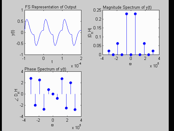
%** Output FS Representation **%
figure(4); clf; % open and clear figure 3
H0 = 0; % DC system gain
y = D0*H0*ones(size(t)); % start out with DC bias term
for n = -N:-1, % loop over negative n
Dn = (1-exp(-j*pi*n))./(j*2*pi*n); % input Fourier coefficient
H = (R/L)*j*n*wo./((j*n*wo).^2 + (R/L)*j*n*wo + 1/(L*C)); % system TF
y = y + real(Dn*H*exp(j*n*wo*t)); % add FS terms
end;
for n = 1:N, % loop over positive n
Dn = (1-exp(-j*pi*n))./(j*2*pi*n); % input Fourier coefficient
H = (R/L)*j*n*wo./((j*n*wo).^2 + (R/L)*j*n*wo + 1/(L*C)); % system TF
y = y + real(Dn*H*exp(j*n*wo*t)); % add FS terms
end;
subplot(2,2,1); plot(t,y); % plot truncated y(t) FS
xlabel('t '); ylabel('y(t)');
title('FS Representation of Output');
%** Output exponential magnitude and phase spectra for 1st 5 harmonics **%
i = 1; % vector index to help store DnH and w
w = 0; Dn = 0; % reinitialize FS variables
for n = -5:-1, % loop over negative n
Dn = (1-exp(-j*pi*n))./(j*2*pi*n); % input Fourier coefficient
H = (R/L)*j*n*wo./((j*n*wo).^2 + (R/L)*j*n*wo + 1/(L*C)); % system TF
DnH(i) = Dn*H; % output Fourier coefficient
w(i) = n*wo; % store associated frequency
i = i + 1; % increment vector index
end;
DnH(i) = D0*H0; w(i) = 0; % store 0 frequency terms
i = i + 1; % increment vector index
for n = 1:5, % loop over positive n
Dn = (1-exp(-j*pi*n))./(j*2*pi*n); % input Fourier coefficient
H = (R/L)*j*n*wo./((j*n*wo).^2 + (R/L)*j*n*wo + 1/(L*C)); % system TF
DnH(i) = Dn*H; % output Fourier coefficient
w(i) = n*wo; % store associated frequency
i = i + 1; % increment vector index;
end;
subplot(2,2,2); % plot magnitude spectrum of y(t)
stem(w,abs(DnH),'filled');
xlabel('\omega ');ylabel('|D_nH|');
title('Magnitude Spectrum of y(t)');
subplot(2,2,3); % plot phase spectrum of y(t)
stem(w,angle(DnH),'filled');
xlabel('\omega '); ylabel('{\angle D_nH} ');
title('Phase Spectrum of y(t)');
Matlab Plots Generated: