EE342: MATLAB M-FILE DEMONSTRATING DIGITAL FILTERING VIA AN IIR FILTER IMPLEMENTED AS A DIFFERENCE EQUATION

%
% Filename:  example14.m
%
% Description:  m-file demonstrating simple digital filter design
%

clear;                      % clear matlab memory
figure(1); clf;             % open and clear figure 1

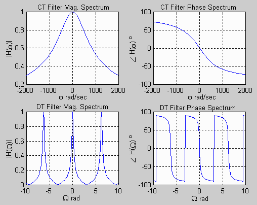
% ** Plot CT Filter Frequency Response **
  w = -2000:0.5:2000;         % CT frequencies to plot H(w)
  Hw = 629.6./(j*w + 629.6);  % CT frequency response
  subplot(2,2,1); plot(w,abs(Hw)); grid;
  xlabel('\omega rad/sec'); ylabel('|H(\omega)|');
  title('CT Filter Mag. Spectrum');

  subplot(2,2,2); plot(w,angle(Hw)*180/pi); grid;
  xlabel('\omega rad/sec'); ylabel('\angle H(\omega) ^o');
  title('CT Filter Phase Spectrum');

% ** Plot DT Filter Frequency Response **
  W = -10:0.05:10;                                    % DT frequencies to plot H(W)
  HW = 629.6*(exp(j*W)+1)./(8629.6*exp(j*W)-7370.4);  % DT frequency response
  subplot(2,2,3); plot(W,abs(HW)); grid;
  xlabel('\Omega rad'); ylabel('|H(\Omega)|');
  title('DT Filter Mag. Spectrum');

  subplot(2,2,4); plot(W,angle(HW)*180/pi); grid;
  xlabel('\Omega rad'); ylabel('\angle H(\Omega) ^o');
  title('DT Filter Phase Spectrum');

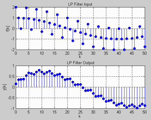
figure(2); clf;             % open and clear figure 2
% ** Define DT Signal to be Filtered **
  k = 0:50;
  fk = cos(0.025*pi*k) + cos(0.5*pi*k);
  subplot(2,1,1); stem(k,fk,'filled'); grid;
  xlabel('k'); ylabel('f[k]');
  title('LP Filter Input');

% ** Filter Signal Via Recursion **
  yprev  = 0; fprev = 0;           % initial values for recursion

  for k = 0:length(fk)-1,          % begin filtering via recursion
    f = fk(k+1);
    y = (7370.4/8629.6)*yprev + (629.6/8629.6)*(f + fprev);

    yprev = y;
    fprev = f;
    yvec(k+1) = y;
    kvec(k+1) = k;
  end;

  subplot(2,1,2);                  % plot filtered signal
  stem(kvec,yvec,'filled'); grid;
  xlabel('k '); ylabel('y[k]');
  title('LP Filter Output');