EE342: MATLAB M-FILE FOR RECURSIVELY SOLVING DIFFERENCE EQUATION APPROXIMATION OF A FIRST ORDER DIFFERENTIAL EQUATION

%
% Filename:  example4.m
%
% Description:  M-file demonstrating discrete-time approximation of a 
%               continuous-time system modeled by a differential
%               equation.
%
  figure(1); clf; clear;                  % clear memory and figure 1

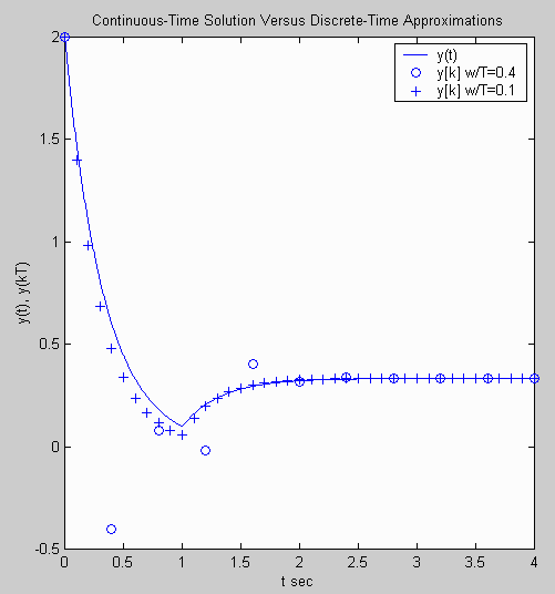
%** Plot exact solution of differential equation **
  t = 0:0.005:4;                          % plot and label CT solution
  y = 2*exp(-3*t)+(1/3)*(1-exp(-3*(t-1))).*(t>=1);
  plot(t,y); hold on;
  xlabel('t sec'); ylabel('y(t), y(kT)');
  title('Continuous-Time Solution And Discrete-Time Approximations');

%** Plot discrete-time approximation using T = 0.4 **
  y_0 = 2.0;                      % initial condition
  kvec(1) = 0; yvec(1) = y_0;     % load ICs into vectors for plotting
  T = 0.4;                        % interval (sample) time
  y_prev = y_0;                   % store IC as previous value of y

  for k = 1:4/T,                  % enter recursion loop
    if(k >= 1+1/T),               % define input 
      f = 1;
    else
      f = 0;
    end;
    y = (1-3*T)*y_prev + T*f;     % update y[k] via difference eqn
    y_prev = y;                   % store value for next iteration
    kvec(k+1) = k;                % store values for plotting
    yvec(k+1) = y;
  end;

  plot(kvec*T, yvec, 'o');

  clear;                          % clear matlab memory

%** Plot discrete-time approximation using T = 0.1 **
  y_0 = 2.0;                      % initial condition
  kvec(1) = 0; yvec(1) = y_0;     % load ICs into vectors for plotting
  T = 0.1;                        % interval (sample) time
  y_prev = y_0;                   % store IC as previous value of y

  for k = 1:4/T,                  % enter recursion loop
    if(k >= 1+1/T),               % define input 
      f = 1;
    else
      f = 0;
    end;
    y = (1-3*T)*y_prev + T*f;     % update y[k] via difference eqn
    y_prev = y;                   % store value for next iteration
    kvec(k+1) = k;                % store values for plotting
    yvec(k+1) = y;
  end;
  
  plot(kvec*T, yvec, '+');
  legend('y(t)','y[k] w/T=0.4','y[k] w/T=0.1'); % label curves