EE342.01: MATLAB M-FILE DEMONSTRATING HOW A DFT CAN BE PADDED WITH ZEROS TO IMPROVE DISCRETE-TIME RESOLUTION

%
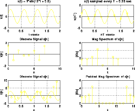
% FILENAME:  example10.m
%
% DESCRIPTION:  m-file for demonstrating padding DFT with zeros to
%               improve resolution of discrete-time signal
%


t = 0:0.01:2.0;                         % generate analog signal
xt = 3*sin(12*t + 0.5);

subplot(3,2,1);                         % plot analog signal
plot(t,xt);
grid;
xlabel('t ');
ylabel('x(t)');
title('x(t) = 3*sin(12*t + 0.5)');

k = 1;                                  % sample analog signal at T=0.25s
for i = 1:25:length(t)-1;
  xn(k) = xt(i);
  k = k + 1;
end;

T = 0.25;                               % plot discrete signal with
n = 0:7;                                % analog signal
xn = xn(1:8);
subplot(3,2,2);
plot(t,xt);
grid;
hold;
stem(n*T,xn);
xlabel('nT ');
ylabel('x(nT)');
title('x(t) sampled every T = 0.25 sec');
hold;

subplot(3,2,3);                         % plot discrete signal again
stem(n,xn);
grid;
xlabel('n');
ylabel('x[n]');
title('Discrete Signal x[n]');

Xk = fft(xn);                           % compute and plot magnitude of
subplot(3,2,4);                         % DFT of discrete signal
stem(n,abs(Xk));
grid;
xlabel('k');
ylabel('|Xk|');
title('Mag Spectrum of x[n]');

Xk = [Xk(1:4) zeros(1,9) Xk(6:8)];      % pad DFT with zeros
xnn = ifft(Xk);                         % compute IDFT to get new signal
n = 0:15;                               

subplot(3,2,6);                         % plot modified (padded) DFT magnitude
stem(n,abs(Xk));
grid;
xlabel('k');
ylabel('|Xk|');
title('Padded Mag Spectrum of x[n]');

subplot(3,2,5);                         % plot new discrete-time signal
stem(n*T/2,xnn/(T/2));                  % with more points
hold;
plot(t,xt);
hold;
grid;
xlabel('n');
ylabel('x[n]');
title('Discrete Signal x[n]');