M-file:
%
% Filename: example1.m
%
% Description: This m-file demonstrates how to
% 1) define and display transfer function and state-space
% model representations,
% 2) plot step responses of systems represented
% in either state-space or transfer function form, and
% 3) convert between state-space and transfer function
% representations.
%
% The DC gearmotor model developed in class is used as
% the example system.
clear; close all; % Clear workspace and close all figures
% Motor parameters:
Jm = 0.01; bm = 0.3; Kt = 0.8;
Ke = 0.8; Ra = 1.4; La = 0.004;
% Gear paramters:
N1 = 10; N2 = 61;
% Load parameters:
Jl = 11; bl = 27;
% Equivalent load seen by motor:
Jt = Jm + (N1/N2)^2*Jl;
bt = bm + (N1/N2)^2*bl;
% State-Space/Variable model definition:
A = [-Ra/La 0 -Ke/La; ...
0 0 1 ; ...
Kt/Jt 0 -bt/Jt];
B = [1/La; 0; 0];
C = [0 0 1];
D = [0];
disp('State-Space Representation by Definition:');
printsys(A, B, C, D);
% Transfer Function model (motor speed)/(armature voltage)
% definition:
numH = Kt; % define numerator and denominator polynomials
denH = conv([La Ra],[Jt bt]) + [0 0 Ke*Kt];
numH = numH/denH(1); % divide numerator and denominator by coefficient
denH = denH/denH(1); % of highest power of s in denominator
disp('Transfer Function by Definition: Omega(s)/Va(s)=');
printsys(numH,denH,'s');
% Determine Transfer Function from State-Space Model using
% built in Matlab function:
[numH2, denH2] = ss2tf(A, B, C, D);
disp('TF from SS via Matlab function: Omega(s)/Va(s)=');
printsys(numH2,denH2,'s');
% Compute State-Space Model from Transfer Function using
% built in Matlab function:
[A2, B2, C2, D2] = tf2ss(numH, denH);
disp('SS from TF via Matlab function:');
printsys(A2, B2, C2, D2);
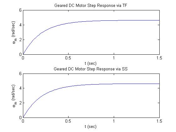
% Plot motor speed response to a 12V step input
ss_sys = ss(A,B,C,D); % create Matlab ss object
tf_sys = tf(numH,denH); % create Matlab tf object
t = 0:0.01:1.5; % define times for step response
[thetamdottf] = 12*step(tf_sys, t); % find step response using tf
subplot(2,1,1); plot(t, thetamdottf); % plot step response
xlabel('t (sec)'); ylabel('\omega_m (rad/sec)');
title('Geared DC Motor Step Response via TF');
[thetamdotss] = 12*step(ss_sys, t); % find step response using ss
subplot(2,1,2); plot(t, thetamdotss); % plot step response
xlabel('t (sec)'); ylabel('\omega_m (rad/sec)');
title('Geared DC Motor Step Response via SS');
Results:
State-Space Representation by Definition:

a =
                        x1           x2           x3
           x1   -350.00000            0   -200.00000
           x2            0            0      1.00000
           x3      2.61763            0     -3.35584


b =
                        u1
           x1    250.00000
           x2            0
           x3            0


c =
                        x1           x2           x3
           y1            0            0      1.00000


d =
                        u1
           y1            0

Transfer Function by Definition:  Omega(s)/Va(s)=

num/den =

             654.4086
   ----------------------------
   s^2 + 353.3558 s + 1698.0725
TF from SS via Matlab function:  Omega(s)/Va(s)=

num/den =

              654.4086 s
   --------------------------------
   s^3 + 353.3558 s^2 + 1698.0725 s
SS from TF via Matlab function:

a =
                        x1           x2
           x1   -353.35584  -1698.07248
           x2      1.00000            0


b =
                        u1
           x1      1.00000
           x2            0


c =
                        x1           x2
           y1            0    654.40860


d =
                        u1
           y1            0
Plots: