M-file:

% Filename:     example3.m
%
% Description:  M-file demonstrating the use of matlab's 
%               rlocus() and rlocfind() functions on the
%               example characteristic equation
%               1 + K(s+2)/(s(s+1)).
%

% clear matlab memory and close all open figures
clear all; close all;

% define numerator and denominator of L(s) and print to check
numL = [1 2];
denL = [1 1 0];
disp(['L(s) = ', poly2str(numL,'s'), '/', poly2str(denL, 's')]);
disp(' ');

% define transfer function object for L(s)
sysL = tf(numL, denL);

% plot closed-loop system's root locus
rlocus(sysL);
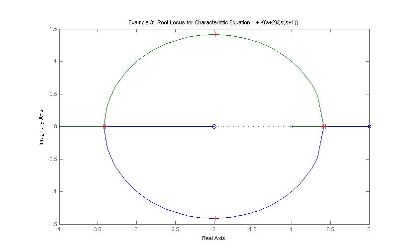
title('Example 3:  Root Locus for Characteristic Equation 1 + K(s+2)/(s(s+1))');

% loop a user-specified number of times to find poles and corresponding
% gains from root-locus plot
nK = input('Enter number of CL-poles on which you wish to click to find corresponding gain, K:  ');
n  = 0;
while(n < nK)
    [K, poles] = rlocfind(sysL)
    n = n + 1;
end;

Matlab Response Generated:

L(s) =    s + 2/   s^2 +  s
 
Enter number of CL-poles on which you wish to click to find corresponding gain, K:  3
Select a point in the graphics window
selected_point =
  -0.5612 - 0.0021i
K =
    0.1712
poles =
   -0.6098
   -0.5613

Select a point in the graphics window
selected_point =
  -3.4020 + 0.0021i
K =
    5.8285
poles =
   -3.4263
   -3.4022

Select a point in the graphics window
selected_point =
  -1.9857 + 1.4158i
K =
    2.9715
poles =
  -1.9857 + 1.4141i
  -1.9857 - 1.4141i

Root-Locus Plot Generated: