M-file:

% File Name:  example4.m
% Description: Comparison of Root-Loci for variety of controllers
%              including P, PD, PI, PID, lead, and lag.
%

% clear matlab memory and close all figures
clear all; close all;

% define motor transfer function, G
L = 1e-3; R = 1; J = 5e-5; B = 1e-4; Ke = 0.1; Kt = 0.1;
numG = [Kt/(L*J)]; denG = [1 (R/L + B/J) (R*B + Ke*Kt)/(L*J) 0];
G    = tf(numG, denG);

% P-control
numD = [1]; denD = [1];
D    = tf(numD, denD);
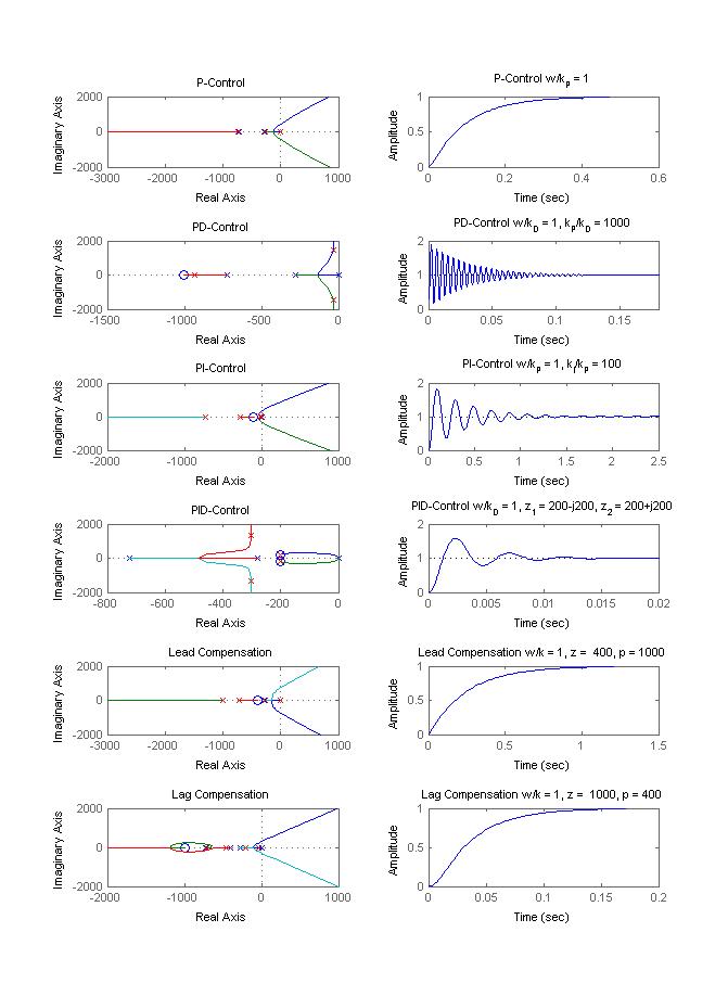
subplot(6,2,1); rlocus(series(D,G)); title('P-Control')
cltf = feedback(series(D,G), [1], -1);
hold on; plot(real(roots(cltf.den{:})), imag(roots(cltf.den{:})), 'rx'); hold off;
subplot(6,2,2); step(cltf); title('P-Control w/k_P = 1');

% PD-control
numD = [1 1000]; denD = [1];
D    = tf(numD, denD);
subplot(6,2,3); rlocus(series(D,G)); title('PD-Control')
cltf = feedback(series(D,G), [1], -1);
hold on; plot(real(roots(cltf.den{:})), imag(roots(cltf.den{:})), 'rx'); hold off;
subplot(6,2,4); step(cltf); title('PD-Control w/k_D = 1, k_P/k_D = 1000');

% PI-control
numD = [1 100]; denD = [1 0];
D    = tf(numD, denD);
subplot(6,2,5); rlocus(series(D,G)); title('PI-Control')
cltf = feedback(series(D,G), [1], -1);
hold on; plot(real(roots(cltf.den{:})), imag(roots(cltf.den{:})), 'rx'); hold off;
subplot(6,2,6); step(cltf); title('PI-Control w/k_P = 1, k_I/k_P = 100');

% PID-control
numD = conv([1 200+200j], [1 200-200j]); denD = [1 0];
D    = tf(numD, denD);
subplot(6,2,7); rlocus(series(D,G)); title('PID-Control')
cltf = feedback(series(D,G), [1], -1);
hold on; plot(real(roots(cltf.den{:})), imag(roots(cltf.den{:})), 'rx'); hold off;
subplot(6,2,8); step(cltf); title('PID-Control w/k_D = 1, z_1 = 200-j200, z_2 = 200+j200');

% Lead-compensation
numD = [1 400]; denD = [1 1000];
D    = tf(numD, denD);
subplot(6,2,9); rlocus(series(D,G)); title('Lead Compensation')
cltf = feedback(series(D,G), [1], -1);
hold on; plot(real(roots(cltf.den{:})), imag(roots(cltf.den{:})), 'rx'); hold off;
subplot(6,2,10); step(cltf); title('Lead Compensation w/k = 1, z =  400, p = 1000');

% Lag-compensation
numD = [1 1000]; denD = [1 400];
D    = tf(numD, denD);
subplot(6,2,11); rlocus(series(D,G)); title('Lag Compensation')
cltf = feedback(series(D,G), [1], -1);
hold on; plot(real(roots(cltf.den{:})), imag(roots(cltf.den{:})), 'rx'); hold off;
subplot(6,2,12); step(cltf); title('Lag Compensation w/k = 1, z =  1000, p = 400');

Root-Locus Plots and Step Responses Generated: