M-file:

% File Name:  example7.m
% Description:  Matlab m-file used to design reference controller
%               for state-space representation of DC motor.
%

% clear matlab memory and close all figures
clear all; close all;

% define motor parameters
L = 1e-3; R = 1; J = 5e-5; B = 1e-4; K = 0.1;

% define motor state variable model
A = [-R/L, 0, -K/L; 0, 0, 1; K/J, 0, -B/J];
B = [1/L; 0; 0];
C = [0, 1, 0];
D = [0];

% check OL motor poles and zeros
ol_poles = eig(A)
ol_zeros = tzero(A,B,C,D)

% design reference controller for motor position with r = 1rad
% begin by placing CL poles of A-BK at -200+j200, -200-j200, -500
K = acker(A,B,[-200+200j, -200-200j, -500])
% find Nx, Nu to map reference value to steady-state input and state
N = inv([A, B; C, D])*[0;0;0;1];
Nx = N(1:3)
Nu = N(4)
% note input voltage is specified by control law u = -Kx + (N_u + KN_x)r,
% use this for real-world implementation

% construct CL-controlled DC motor model for simulation
Ap = A - B*K;
Bp = B*(Nu + K*Nx);
Cp = C - D*K;
Dp = D*(Nu + K*Nx);
clsys = ss(Ap,Bp,Cp,Dp);

% check CL poles and zeros
cl_poles = eig(Ap)
cl_zeros = tzero(Ap,Bp,Cp,Dp)

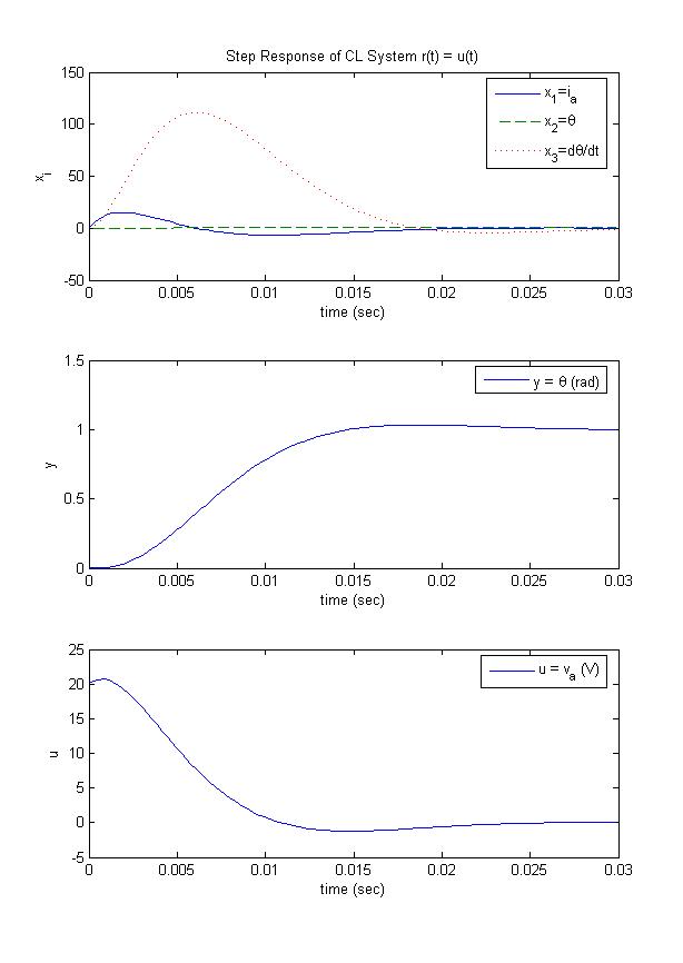
% simulate step response for r = 1rad
[y, t, x] = step(clsys);
figure(1);
subplot(3,1,1); plot(t,x(:,1),'-',t,x(:,2),'--',t,x(:,3),':');
legend('x_1=i_a', 'x_2=\theta', 'x_3={d\theta/dt}');
xlabel('time (sec)'); ylabel('x_i');
title('Step Response of CL System r(t) = u(t)');
subplot(3,1,2); plot(t,y); legend('y = \theta (rad)');
xlabel('time (sec)'); ylabel('y');
subplot(3,1,3); plot(t, -K*x.' + (Nu + K*Nx)*1); legend('u = v_a (V)');
xlabel('time (sec)'); ylabel('u');

Matlab Response:

ol_poles =
         0
 -722.3617
 -279.6383

ol_zeros =
   Empty matrix: 0-by-1

K =
   -0.1020   20.0000    0.0391

Nx =
     0
     1
     0

Nu =
     0

cl_poles =
  1.0e+002 *
  -5.0000          
  -2.0000 + 2.0000i
  -2.0000 - 2.0000i

cl_zeros =
   Empty matrix: 0-by-1

Step Response Generated: