Initial Matlab Commands (before running Simulink):

% clear matlab memory and close all figures
clear all; close all;

% define motor parameters
L = 1e-3; R = 1; J = 5e-5; B = 1e-4; K = 0.1;

% define motor state variable model
A = [-R/L, 0, -K/L; 0, 0, 1; K/J, 0, -B/J];
B = [1/L; 0; 0];
C = [0, 1, 0];
D = [0];

% check observability
O = obsv(A,C);
rank(O)

% design observer by placing poles of A-LC at -500+j250, -500-j250, -200
Lt = acker(A.',C.',[-500+250j, -500-250j, -2000]);
L  = Lt.'

% check poles of estimator-error dynamics
est_poles = eig(A - L*C)

% redefine C,D to get all states out of DC motor block -
% use only y = x_2 for observer
C = [1, 0, 0; 0, 1, 0; 0, 0, 1];
D = [0; 0; 0];

% define DC motor intial conditions for use in Simulink
x0 = [0, 0, 0];

% define estimator state variable model and initial conditions
Ahat = A;
Bhat = [B, L];
Chat = [1, 0, 0; 0, 1, 0; 0, 0, 1];
Dhat = [0, 0; 0, 0; 0, 0];
xhat0 = [5, 5, 5];

Matlab Response:

ans =
     3

L =
       56450
        1998
      108504

est_poles =
  1.0e+003 *
  -0.5000 + 0.2500i
  -0.5000 - 0.2500i
  -2.0000   

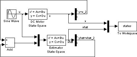
Simulink File

Matlab Plot Commands (after Simulink):

figure(1);
subplot(3,1,1); plot(tout, states(:,1), tout, states(:,4), '--');
xlabel('time (sec)'); legend('x_1 = i_a', 'xhat_1');
title('States x and their Estimates xhat');
subplot(3,1,2); plot(tout, states(:,2), tout, states(:,5), '--');
xlabel('time (sec)'); legend('x_2 = \theta', 'xhat_2');
subplot(3,1,3); plot(tout, states(:,3), tout, states(:,6), '--');
xlabel('time (sec)'); legend('x_3 = \theta_{dot}', 'xhat_3');

Plots Generated: