M-file:

% Filename:     rootlocus.m
%
% Description:  M-file demonstrating the use of matlab's 
%               rlocus() and rlocfind() functions on the
%               example characteristic equation
%               1 + K(s+2)/(s(s+1)).
%

% clear matlab memory and close all figures
clear all; close all;

% define numerator and denominator of L(s) and print to check
numL = [1 2]; denL = [1 1 0];
disp(['L(s) = ', poly2str(numL,'s'), '/', poly2str(denL, 's')]);
disp(' ');

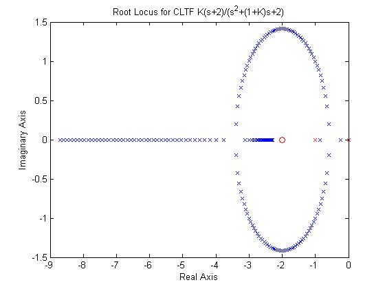
%***** First Approach to Root Locus - Loop Over K *****

% open figure 1
figure(1);

% find open loop zeros and plot as o's, 
% find open loop poles and plot as x's
olzeros = roots(numL);
olpoles = roots(denL);
plot(real(olzeros),imag(olzeros),'ro'); hold on;
plot(real(olpoles),imag(olpoles),'rx');

% loop over K, find and plot closed-loop poles
for K = 0.1:0.1:10,
    clpoles = roots([1, 1+K, 2*K]);
    plot(real(clpoles),imag(clpoles),'bx');
end
hold off;
xlabel('Real Axis'); ylabel('Imaginary Axis');
title('Root Locus for CLTF K(s+2)/(s^2+(1+K)s+2)');

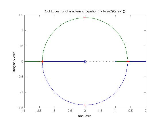
%***** Second Approach to Root Locus - Use rlocus() and rlocfind() *****

% open figure 2
figure(2);

% define transfer function object for L(s)
sysL = tf(numL, denL);

% plot closed-loop system's root locus
rlocus(sysL);
title('Root Locus for Characteristic Equation 1 + K(s+2)/(s(s+1))');

% loop a user-specified number of times to find poles and corresponding
% gains from root-locus plot
nK = input('Enter number of CL-poles on which you wish to click to find corresponding gain, K:  ');
n  = 0;
while(n < nK)
    [K, poles] = rlocfind(sysL)
    n = n + 1;
end

Matlab Response Generated:

>> rootlocus
L(s) =    s + 2/   s^2 +  s
 
Enter number of CL-poles on which you wish to click to find corresponding gain, K:  3
Select a point in the graphics window

selected_point =
  -0.5829 - 0.0047i
K =
    0.1716
poles =
  -0.5858 + 0.0037i
  -0.5858 - 0.0037i

Select a point in the graphics window
selected_point =
  -2.0047 + 1.4115i
K =
    3.0095
poles =
  -2.0048 + 1.4142i
  -2.0048 - 1.4142i

Select a point in the graphics window
selected_point =
  -3.4076 - 0.0047i
K =
    5.8284
poles =
   -3.4189
   -3.4095

Root-Locus Plots Generated: