EE 570: Example of Trajectory Generation

Cubic, Quintic and Linear Segment with Parabolic Blend

M-File:

% Example of trajectory generation
% Filename:  gentraj.m

clear all; close all; clc; % clear memory, figures, and window

% ** Cubic Polynomial Trajectories **
% intial time, joint value and joint velocity
to = 5; qo = 0.5;  qdoto = 0;
% final time, joint value and joint velocity
tf = 12; qf = -0.7; qdotf = 0; 
% Coefficient matrix for cubic trajectory and its derivative
% at initial and final joint values.
A = [1,  to,  to^2, to^3;   ...
     0,  1,   2*to, 3*to^2; ...
     1,  tf,  tf^2, tf^3;   ...
     0,  1,   2*tf, 3*tf^2];
% Vector of intial and final joint positions and velocities
b = [qo; qdoto; qf; qdotf];
% Compute coefficients of trajectory polynomial using
% notion of a = inv(A)*b, but using Gaussian Elimination
a = A\b;
% Evaluate cubic polynomial at times
t = to:(tf-to)/500:tf;
q     = a(1) + a(2)*t + a(3)*t.^2 + a(4)*t.^3;
qdot  = a(2) + 2*a(3)*t + 3*a(4)*t.^2;
qddot = 2*a(3) + 6*a(4)*t;
% Plot trajectories
figure(1);
subplot(2,2,1);
plot(t,q,'b-',t,qdot,'g--',t,qddot,'r-.','LineWidth',2);
legend('q','dq/dt','d^2q/dt^2');
xlabel('time (sec)'); ylabel('Joint Trajectory');
title('Trajectory using Cubic Polynomial');

% ** Quintic Polynomial Trajectories **
clear all;
% intial time, joint value, joint velocity and joint acceleration
to = 5; qo = 0.5; qdoto = 0; qddoto = 0;
% final time, joint value, joint velocity and joint acceleration
tf = 12; qf = -0.7; qdotf = 0; qddotf = 0;
% Coefficient matrix for quintic trajectory and its derivative
% at initial and final joint values.
A = [1,  to,  to^2, to^3,   to^4,    to^5;   ...
     0,  1,   2*to, 3*to^2, 4*to^3,  5*to^4;   ...
     0,  0,   2,    6*to,   12*to^2, 20*to^3; ...
     1,  tf,  tf^2, tf^3,   tf^4,    tf^5;   ...
     0,  1,   2*tf, 3*tf^2, 4*tf^3,  5*tf^4;   ...
     0,  0,   2,    6*tf,   12*tf^2, 20*tf^3];
% Vector of intial and final joint positions and velocities
b = [qo; qdoto; qddoto; qf; qdotf; qddotf];
% Compute coefficients of trajectory polynomial using
% notion of a = inv(A)*b, but using Gaussian Elimination
a = A\b;
% Evaluate quintic polynomial at times
t = to:(tf-to)/500:tf;
q     = a(1) + a(2)*t + a(3)*t.^2 + a(4)*t.^3 + a(5)*t.^4 + a(6)*t.^5;
qdot  = a(2) + 2*a(3)*t + 3*a(4)*t.^2 + 4*a(5)*t.^3 + 5*a(6)*t.^4;
qddot = 2*a(3) + 6*a(4)*t + 12*a(5)*t.^2 + 20*a(6)*t.^3;
% Plot trajectories
subplot(2,2,2);
plot(t,q,'b-',t,qdot,'g--',t,qddot,'r-.','LineWidth',2);
legend('q','dq/dt','d^2q/dt^2');
xlabel('time (sec)'); ylabel('Joint Trajectory');
title('Trajectory using Quintic Polynomial');

% ** Linear Segments with Parabolic Blends (PSPB) **
clear all;
% intial time, joint value and joint velocity
to = 0; qo = 0.5;
% final time, joint value and joint velocity
tf = 7; qf = -0.7;
% constant velocity and blend time
V = -0.2; tb = (qo - qf + V*tf)/V;
% check that V is within limits
Vmin = (qf - qo)/tf;
if (V > Vmin || V < 2*Vmin) % this check assumes V negative
    display(['V = ',num2str(V), ' is not within limits',...
            '(',num2str(Vmin),', ',num2str(2*Vmin),')']);
    display('LSPB will not be correct!');
end;
a(1) = qo; a(2) = 0; a(3) = V/(2*tb);
b(1) = qf - (V*tf^2)/(2*tb); b(2) = V*tf/tb; b(3) = -V/(2*tb);

% ** Linear Segments with Parabolic Blends (PSPB) **
% Begin with unshifted version on t = [0, 7].
t = to:(tf-to)/500:tf;
q = (a(1) + a(2)*t + a(3)*t.^2).*(t<=tb) + ...
    ((qf + qo - V*tf)/2 + V*t).*((t>tb)-(t>=(tf-tb))) + ...
    (b(1) + b(2)*t + b(3)*t.^2).*(t>(tf-tb));
qdot = (a(2) + 2*a(3)*t).*(t<=tb) + ...
       V.*((t>tb)-(t>=(tf-tb))) + ...
       (b(2) + 2*b(3)*t).*(t>(tf-tb));
qddot = 2*a(3)*(t<=tb) + ...
        0*((t>tb)-(t>=(tf-tb))) + ...
        2*b(3)*(t>(tf-tb));
subplot(2,2,3);
plot(t,q,'b-',t,qdot,'g--',t,qddot,'r-.','LineWidth',2);
legend('q','dq/dt','d^2q/dt^2');
xlabel('time (sec)'); ylabel('Joint Trajectory');
title('(Unshifted) Trajectory using LSPB');

% ** Linear Segments with Parabolic Blends (PSPB) **
% Now shift over to match desired time interval t = [5, 12]
% remembering to use t = t - 5 in time functions.
ts = 5; t = t + ts;
q = (a(1)+a(2)*(t-ts)+a(3)*(t-ts).^2).*((t>=ts)-(t>=(tb+ts))) + ...
    ((qf + qo - V*tf)/2 + V*(t-ts)).*((t>(tb+ts))-(t>=(tf-tb+ts))) + ...
    (b(1) + b(2)*(t-ts) + b(3)*(t-ts).^2).*(t>(tf-tb+ts));
qdot = (a(2) + 2*a(3)*(t-ts)).*(t<=(tb+ts)) + ...
       V.*((t>(tb+ts))-(t>=(tf-tb+ts))) + ...
       (b(2) + 2*b(3)*(t-ts)).*(t>(tf-tb+ts));
qddot = 2*a(3)*(t<=(tb+ts)) + ...
        0*((t>(tb+ts))-(t>=(tf-tb+ts))) + ...
        2*b(3)*(t>(tf-tb+ts));
subplot(2,2,4);
plot(t,q,'b-',t,qdot,'g--',t,qddot,'r-.','LineWidth',2);
legend('q','dq/dt','d^2q/dt^2');
xlabel('time (sec)'); ylabel('Joint Trajectory');
title('(Shifted) Trajectory using LSPB');

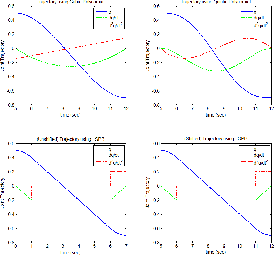
Figure generated showing trajectories: