EE 544: Modern Control Theory
Instructor: Kevin Wedeward, office: Workman 221, phone: 835-5708,
e-mail: wedeward@ee.nmt.edu, web-page: www.ee.nmt.edu/~wedeward/
Class Time/Place: T 09:00am-11:30am in Workman 117
Office Hours: MWF 09:00am-10:00am, 11:00am-12:00pm
Textbook:
- A preprint of Feedback Systems: An Introduction
for Scientists and Engineers by Karl J. Åström and
Richard M. Murray will be made available to students.
- The authors' companion website for the textbook can be found
here.
Prerequisites: Courses in and/or knowledge of
Linear Systems, Laplace Transforms, Complex Numbers,
Linear Algebra, and Ordinary Differential Equations.
Description: EE 544 is intended for
advanced engineering students who are interested in learning the
principles of design and analysis for feedback systems.
Objective: Develop an understanding of feedback
control systems to include: concepts, terminology, modeling,
analysis and synthesis.
Topics: Chapters 1-12 of textbook.
Grading:
- Homework: 20%
- Homework will generally be assigned weekly.
- Collaboration with other students is encouraged; however, the work turned in must be your own.
- Participation: 15%
- Two Quizzes: 25%
- Labs/Projects: 20%
- Paper Review: 20%
Reading Assignments:
- Read Chapters 1 and 2 (08/21/2007)
- Read Chapters 3 and 4 (08/28/2007)
- Read Chapter 5 (09/04/2007)
- Read Chapter 6 (09/11/2007)
- Read Chapter 7 (09/25/2007)
- Read Chapter 8 (10/09/2007)
- Read Chapter 10 and material on root locus
Coursework:
- Paper review is due M 12/10/2007 with paper selection by T 11/06/2007.
Additional guidelines can be found here.
- Project 1 due T 10/30/2007
- Lab 1 (SBC-Linux-DAC-C) due T 11/06/2007
- Project 2 due F 11/30/2007
- Lab 2 (State-space control and observer) due F 12/07/2007
- Lab 3 (PID controller) due F 12/07/2007
Homework:
- Homework 1 due T 08/28/2007:
- Exercise 1.2 - look at two examples (versus five): 1) Internet Transmission Control Protocol (TCP)
reliability and congestion control, and 2) feedback control system taken from your
experience and interest.
- Exercise 1.6
- Homework 2 due T 09/04/2007: Exercises 2.1, 3.1, 3.4, 3.11
- Homework 3 due T 09/11/2007: For both Exercise 4.13 and problem in handout
(choose l = 1.00m, g = 9.81m/s, R = 0.10m if you haven't already picked
other values) -
- put nonlinear system model in state-space/variable form
- show vector field and sample phase portraits for nonlinear model
- find equilibrium points
- linearize system about equilibrium points
- show vector fields and sample phase portraits for linearized systems
- compute eigenvalues for linearized systems
- comment on system stability (both linear and nonlinear)
- Homework 4 due T 09/18/2007:
- Exercise 4.10 with simulation
- Simulate pendulum in class example with PD-plus-gravity compensation
control
- Homework 5 due T 09/25/2007: Handout
- Homework 6 due T 10/09/2007: Work Examples 6.5, 6.7
- Homework 7 due T 10/23/2007: Using inverted pendulum example (6.7)
a) implement LQR control, b) add observer using cart position as
output, c) show y->r, xhat->x in plots
- Homework 8 due T 11/13/2007: Problems 5.4d, 5.7c, 5.12 in handout.
Sketch by hand following rules (where reasonable) and plot with Matlab.
- Homework 9 due T 11/20/2007:
- Plot root-locus for class example and controllers presented to confirm sketches;
- Choose controllers (and associated gains) based upon root-locus that
indicate feasible controllers;
- Simulate step responses for selected controllers and gains;
- Comment on how close responses are to meeting specifications
and steady-state error predictions.
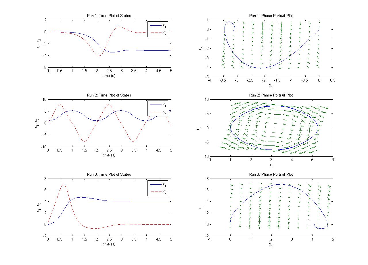
Examples:
- M-files pendulum.m and fpendulum.m
used to find pendulum time responses, vector fields, and phase portraits shown in
this figure.
- Matlab example to plot root-locus by looping
over parameter values or using rlocus() and rlocfind() functions.
Resources: